Review of Austrian Economics

Some Austrian Perspectives on Keynesian Fiscal Policy and the Recovery in the Thirties

Gene Smiley

The standard explanation for the snail-like pace of the recovery from the Great Depression was first proposed by E. Cary Brown in 1956, and was enhanced and extended by Larry Peppers in 1973.1 Though there are a few skeptics, the story of the federal government’s failure to use expansionary fiscal policy is repeated in most economic history, principles of economics, and intermediate macroeconomics textbooks.2 Here, I suggest that this tale is wrong since it is built upon assumptions inconsistent with observed behavior during the recovery from the Great Depression. Using some insights from Austrian analysis, I conclude that a more expansionary fiscal policy would have had little effect in promoting a more rapid recovery from the Depression.

Brown and Peppers argued that the reason for the retarded recovery in the 1933–39 period was that the federal government failed to use expansionary fiscal policy.3 This is not to say that federal government expenditures did not increase.4 Rather, Brown and Peppers argued that the problem was that both the Hoover and Roosevelt administrations also sharply increased tax rates in attempting to “balance” the federal government’s budget. The contractionary effects of increasing taxes largely offset the expansionary effects of increasing spending. With the exception of 1931 and 1936, when the federal government made “bonus” payments to veterans, Peppers’s analysis indicated that the federal budget would have shown a substantial surplus if full employment had prevailed.5 Both Brown and Peppers argued that the appropriate policy would have been to increase federal spending without increasing taxes. Such a policy, they contended, would have increased aggregate demand and, through the Keynesian spending multiplier, more quickly restored full employment.

Apparently Brown and Peppers assumed that the money borrowed to finance such a federal government deficit would not have crowded out other spending. In Keynesian analysis, this requires that there be a highly interest-elastic demand for money balances—something approaching a Keynesian liquidity trap. Alternatively, the Federal Reserve System could have purchased the additional federal government debt and created new money by an equal amount. If the reason for the contraction was an insufficient stock of money, then the new money could have employed the idle resources without causing inflation or reducing real spending in any other sector in the economy.

Though the stock of money did increase from 1933 through 1939, this was due to the flow of gold into the United States, not to the actions of the Federal Reserve System. Since the FRS did not aid the federal government’s financing of its deficit, and, in fact, consistently attempted to reduce the growth of the money stock, I do not consider the monetization of the deficit a viable alternative. One aspect of the question of the potential power of fiscal policy then concerns crowding out as a result of the deficit spending. My purpose in the first part of this article is to establish plausible explanations of what might have happened to the funds collected through increased taxes and increased borrowing if the government had not gained the additional funds and increased spending. This provides one part of the answer to the question of what would have been the effect of greater deficit spending by the federal government by addressing the question from the perspective of the Keynesian analysis.

In the second part of the article, I consider the question of the potential effect of greater deficit spending by the federal government during the 1930s recovery from the perspective of Austrian analysis. The procedure here is to consider the effect of increased federal spending on the structure of relative prices, an effect Keynesians and monetarists generally tend to ignore.

In 1942, the U.S. National Resources Planning Board estimated that for the 1933–39 period, 42.6 percent of the federal public aid expenditures were financed by tax revenues, and 57.4 percent financed by additional debt issues.6 Whether financed by tax increases or additional bond sales, if the positive spending multiplier occurs, it is because some of the increased taxes or purchases of additional debt use money that otherwise would have been completely idle, or would not have existed.7

For federal spending financed by equivalent tax increases, the size of the Keynesian fiscal spending multiplier depends on the type of savings reduced by the tax increase.8 Prior to World War II, Milton Friedman and Anna Schwartz’s data show that the deposit/currency ratio fell to a low of just under 5 in 1933, and rose to 7.25 by early 1937.9 Households generally held the bulk of their savings as time deposits in financial intermediaries, while demand deposit and cash holdings were largely related to household transactions.10 The argument that banks relent most of the deposited funds will be developed here. Therefore, if the tax increase induced individuals to reduce savings by decreasing bank deposits, this would have brought about a nearly proportionate reduction in bank lending and private sector spending.11 Even if the tax increase proportionately reduced household deposit and currency “savings,” the fact that households only held $1 in currency for every $5 to $7.25 in deposits means that the fiscal multiplier would have been tiny.12 Considering that household currency holdings were largely related to transactions demands and the progressive personal income tax system, it seems most likely that during the 1933–39 period, the federal government spending financed by equivalent tax increases would have had a multiplier close to zero—certainly not close to one.

The majority of the federal government’s public aid expenditures, 57.4 percent, were financed by selling debt. Table 1 presents the ownership of the federal debt between 1933 and 1939 and the six-month (or yearly) changes in the amount held. The data show that there was virtually no monetization of the debt, especially from June 1934 on.13 From June 1933 through December 1939, 74.7 percent of the total debt issued was purchased by member and nonmember banks, savings banks, insurance companies, and “other investors”—a category that includes other financial firms, all nonfinancial firms, all households, and any other investors. Nearly 89 percent of all the federal debt sold in the private sector was sold to banks and insurance companies. For the federal government expenditures financed by debt sold to the private sector to have a large multiplier effect, much of the debt must have been purchased by banks which largely used reserves that otherwise would not have been used for any purpose other than idle excess bank reserves, by insurance companies which mainly used money that otherwise would have been held only as idle currency balances outside of the banking system, and by “other investors” who primarily used money that otherwise would have been held as idle currency—not bank deposit—balances.

I will first examine the behavior of nonfinancial firms and individuals (“Other investors”).14 As noted, the deposit/currency ratio rose from 5 to 7.25 between 1933 and 1937, where it roughly remained for the rest of the decade. Recent empirical research suggests that there was a highly interest-inelastic demand for money balances during this period.15 Money market and securities market interest rates (such as those on treasury bills, U.S. government and corporate bonds, major city bank commercial loans, prime commercial paper, and stock exchange time loans) were very low and relatively stable or falling slightly. Though bank commercial loans rates, outside of the largest cities, were higher and tended to rise from 1934 to 1936, particularly in the western states, the newly controlled deposit rates were low and could not rise.16 With the roughly constant interest rates, the interest-inelastic demand for money balances, and the fact that households and firms held from $5 up to $7.25 of deposit balances for every dollar of currency, it seems most unlikely that any significant portion of the debt sold to those in the “other investors” category would have been purchased using idle currency balances.

Table 1
Ownership of U.S. Government Debt, 1933–39 (end-of-month figures in $ millions)
Date	Total Amount Outstanding	Federal Agencies and Trust Funds	Federal Reserve Banks	FRS Member Banks	Other Commercial Banks	Mutual Savings Banks	Insurance Companies	Other Investors
6/1933	22,158	690	1,988	6,887	590	720	1,000	10,300
6/1934	27,161	1,428	2,432	9,413	900	970	1,500	10,500
6/1935	31,768	1,991	2,433	11,430	1,290	1,540	2,600	10,500
6/1936	37,707	2,320	2,430	13,672	1,600	2,050	3,900	11,700
12/1936	38,362	2,432	2,430	13,545	1,790	2,250	4,500	11,400
6/1937	40,465	3,584	2,526	12,689	1,870	2,390	5,000	12,400
12/1937	41,353	4,255	2,564	12,372	1,780	2,450	5,300	12,600
6/1938	41,428	4,777	2,564	12,343	1,700	2,690	5,500	11,900
12/1938	43,891	5,333	2,564	13,223	1,850	2,880	5,700	12,300
6/1939	45,336	5,886	2,551	13,777	1,920	3,040	5,900	12,300
12/1939	47,067	6,531	2,484	14,328	1,970	3,100	6,300	12,400
Changes in the Amount of U.S. Government Securities Owned
6/33 to 6/34	5,003	738	444	2,526	310	250	500	200
6/34 to 6/35	4,607	563	1	2,017	390	570	1,100	0
6/35 to 6/36	5,939	329	-3	2,242	310	510	1,300	1,200
6/36 to 12/36	655	112	0	-127	190	200	600	-300
12/36 to 6/37	2,103	1,152	96	-856	80	140	500	1,000
6/37 to 12/37	888	671	38	-317	-90	60	300	200
12/37 to 6/38	75	522	0	-29	-80	240	200	-700
6/38 to 12/38	2,463	556	0	880	150	190	200	400
12/38 to 6/39	1,445	553	13	554	70	160	200	0
6/39 to 12/39	1,731	645	-7	551	50	60	400	100

Source: Board of Governors of the Federal Reserve System, Banking and Monetary Statistics (Washington, D.C.: National Capital Press, 1943), table 149, p. 512.

Note: Components may not add to the total due to the rounding of the estimates. The estimated figures for “other commercial banks” and “mutual savings banks” were rounded to the nearest $10 million and the estimated figures for “insurance companies” and “other investors” were rounded to the nearest $100 million.

The evidence suggests similar behavior for insurance companies. In the interwar years, the ten largest life insurance companies operated with very low ratios of cash balances to total assets. The ratio averaged about 0.7 to 0.8 percent in the twenties, about 2.0 percent in the thirties after the Depression, and from 1.0 to 1.5 percent from 1947 to 1955.17 The cash balances included both bank deposits and currency. Though the data on this composition are not available, surely the insurance companies would have held the bulk of their “cash” balances as bank deposits rather than currency on hand since bank deposits were the most efficient means of making payments to claimants, policyholders, agents, and employees. Table 1 shows that insurance companies increased their holdings of federal government debt by over $1 billion a year from June 1934 through June 1937.

If the insurance companies had not purchased the additional government debt, would they have held these funds in idle cash balances rather than purchasing any private or nonfederal government financial securities; if held as cash balances, would the money have been held mainly as currency holdings rather than as bank deposits? The most plausible answer to both of these questions would seem to be no. First, the life insurance companies were contractually obligated to make future payments. Surely, if they had not invested in federal government debt, they would have invested in private or local and state government financial securities. Second, even if they would have held all of the funds as “cash” balances (rather than purchasing the new issues of federal debt), it seems most reasonable to assume that they would have held most of the “cash” in bank deposits rather than currency.

Williamson and Smalley’s data on Northwestern Mutual Life make possible some instructive calculations for that large life insurance company. Northwestern Mutual’s “cash” holdings were $10.3 million in 1933, $10 million in 1935, and $14.0 million in 1939, or 1.03, 0.93, and 1.08 percent respectively of the admitted assets. Northwestern’s holdings of U.S. government securities can roughly be estimated at $25 million dollars in 1935, $150 million in 1935, and $125 million in 1939. If the U.S. government securities had not been issued and Northwestern had then held additional cash balances of $125 and 100 million in 1935 and 1939, their cash as a percentage of admitted assets would have been 12.59 percent in 1935, and 8.82 percent in 1939. This behavior hardly seems plausible.

In his history of the Metropolitan Life Insurance Company, Louis Dublin indicated that a reduced supply of other investment opportunities, as well as the much lower risk associated with federal government debt, led insurance companies to purchase more federal bonds in the post-1933 period.18 In their history of Northwestern Mutual Life, Williamson and Smalley provided more information on this company’s investments during the thirties. The company built up its holdings of federal government bonds in 1934 and 1935, “when the supply of higher yielding securities was limited” (emphasis added).19 However, the absolute and relative amount of U.S. government bonds held by Northwestern Mutual Life declined from 1935 through 1941. Williamson and Smalley report that the company’s investment management felt that “the most promising areas for an expansion of the Company’s security holdings were state, county, and municipal bonds in the United States and the obligations in public utilities and industrial concerns.”20 They report that rather than wait for applications to come to them, the company actively sought out these types of investments. The state, county, and municipal bonds were, of course, tax exempt. According to Williamson and Smalley, Northwestern considered public utility and industrial securities the most attractive investments “largely because of their favorable showing during the Depression and their future prospects.”21

This analysis does not suggest that the insurance companies would have held all or even much of the assets used to purchase the federal debt as idle currency balances if the additional federal debt had not been issued.

The behavior of the banks was critical since they were the dominant purchasers of the federal debt and controlled the deposited funds of insurance companies, other nonbank financial firms, and other investors. From June 1933 through December 1939, 60.2 percent of the additional U.S. debt purchased by the private sector was purchased by member and nonmember commercial banks and savings banks. For federal spending to have a large multiplier effect, as the Keynesian scenario suggests, the banks must have purchased the debt largely using funds that otherwise would have been held only as idle excess bank reserves. Friedman and Schwartz have calculated that the ratio of bank reserves to bank deposits for all banks rose continuously from 1933 through 1939.22 Though at the time, the Federal Reserve Board asserted that the accumulating excess reserves resulted from inadequate loan demand at any reasonable interest rate, Friedman and Schwartz have argued that bankers were consciously building up the excess reserves as additional liquidity; in effect, a “Maginot line” of excess reserves against further banking crises. If the excess reserves were desired by bankers, then the purchase of federal government debt would have been made in lieu of loans and other securities purchases, rather than have been made using funds that otherwise would have been held only as idle excess reserves.

It is difficult to determine the motives of the managers of the banks. However, there are some data and clues upon which to base an analysis. In the first two years after the trough of the Depression, banks were heavy purchasers of the bonds being sold by the federal government to finance the New Deal programs. FRS member banks increased their holdings of U.S. government securities by 50.7 percent from June 1933 through June 1935, nonmember banks increased their holdings of these securities by 78.2 percent in this period, and mutual savings banks increased these holdings by 75.7 percent. Member and nonmember banks’ holdings of other securities rose by only 7.4 percent and 2.9 percent respectively in this two-year period, while mutual savings banks’ holdings of other securities fell. The loans of all of these banks fell during these two years. These figures are shown in table 2.

Rates on government bonds, industrial bonds, commercial paper, and New York City bank loans were very low in absolute terms, and falling through early 1935. This has led to suggestions that the demand for loans and for investment funds in the immediate post-Depression years was so low that if the federal government had not sold securities to finance its spending, banks, individuals, and firms would have had no choice but to hold larger idle money or reserve balances. However, there is evidence against this assertion. When bank loan rates for banks outside of the major financial centers are examined, one finds that loan rates were much higher and actually rose sharply in a number of western states in the two and a half years after the trough of the Depression.23 The rising interest rates would not suggest such inadequate loan demand.

Table 2
Loans and Securities Held by FRS Member, Nonmember Commercial, and Mutual Savings Banks (end-of-month figures in $ millions)
	Loans			U.S. Securities			Other Securities
Date	FRS Member Banks	Nonmember Commercial Banks	Mutual Savings Banks	FRS Member Banks	Nonmember Commercial Banks	Mutual Savings Banks	FRS Member Banks	Nonmember Commercial Banks	Mutual Savings Banks
6/33	12,858	3,491	5,894	6,887	589	723	5,041	1,491	3,331
12/33	12,833	3,491	5,808	7,254	na	na	5,132	na	na
6/34	12,513	3,177	5,606	9,413	895	895	5,239	1,495	3,233
12/34	12,028	2,960	5,451	10,895	na	na	5,227	na	na
6/35	11,928	2,981	5,304	11,430	1,287	1,542	5,427	1,535	2,913
12/35	12,175	2,944	5,183	12,269	na	na	5,542	na	na
6/36	12,541	3,017	5,077	13,672	1,598	2,052	6,045	1,666	2,713
12/36	13,360	2,998	5,001	13,545	1,789	2,253	6,095	1,685	2,719
6/37	14,284	3,147	4,978	12,689	1,874	2,391	5,765	1,712	2,724
12/37	13,958	3,142	4,965	12,371	1,784	2,454	5,423	1,655	2,675
6/38	12,937	3,115	4.929	12,343	1,699	2,685	5,440	1,574	2,489
12/38	13,207	3,156	4,897	13,223	1,848	2,883	5,640	1,594	2,382
6/39	13,141	3,282	4,897	13,777	1,923	3,043	5,686	1,559	2,309
12/39	13,962	3,281	4,926	14,329	1,971	3,102	5,651	1,474	2,190
Changes for the Six Months Ending
12/33	-20	-78	-86	367	153a	124a	91	2a	-49a
6/34	-320	-326	-202	2,159	153a	124a	107	2a	-49a
12/34	-485	-217	-155	1,482	196a	285a	-12	20a	-160a
6/35	-100	21	-147	535	196a	285a	200	20a	-160a
12/35	247	-37	-121	839	155a	255a	115	65a	-100a
6/36	366	73	-106	1,403	156a	255a	503	65a	-100a
12/36	819	-19	-76	-127	191	201	50	21	6
6/37	924	149	-23	-856	85	138	-330	27	5
12/37	-326	-5	-13	-318	-90	63	-342	-57	-4
6/38	-1,021	-27	-36	-28	-85	231	17	-81	-186
12/38	270	41	-32	880	149	198	200	20	-107
6/39	-66	126	0	554	75	160	46	-35	-73
12/39	821	-1	29	552	48	59	-35	-85	-119

Source: Board of Governors of the Federal Reserve System, Banking and Monetary Statistics (Washington, D.C.: National Capital Press, 1943), tables 4–7, pp. 20–23. na: not available.

aOver these dates only the twelve-month change could be calculated. Thus, these figures for the six-month changes are one-half of the twelve-month changes.

In addition, there is also evidence that banks rationed credit by simply refusing to make some loans. Ben Bernanke examined this evidence as part of his study of how the financial crises of the Depression raised the costs of credit intermediation and reduced the efficiency of the financial sector.24 Lewis Kimmel’s survey of credit availability during 1933–38 indicated that a large share of manufacturing firms were refused bank loans during this period; in particular, more than 30 percent of the smaller manufacturing firms reported being refused credit.25 Relatively few of the largest manufacturing firms reported difficulty in securing bank loans. A survey of firms in the seventh Federal Reserve District in 1934–35 found “a genuine unsatisfied demand for credit by solvent borrowers,” and a U.S. Dept. of Commerce survey of small firms with high credit ratings found that nearly half of them had difficulty borrowing for working capital and most were not able to obtain investment funds.26

This suggests that in the first two to two and a half years after the end of the Depression, banks were investing in the new issues of government securities because of the extremely low risks involved in holding these “safe” financial assets compared to alternatives, not because there were simply no other investment or loan opportunities. Under these circumstances, if the additional federal government bonds had not been issued, then banks would have turned, perhaps reluctantly, to other investments and loan demands. Private and nonfederal government spending was forced to decline because of the federal government’s increased spending.

As economic activity began to recover, the authorities of the Federal Reserve System became increasingly concerned about the buildup of banks’ excess reserves. They feared that with the revival of the demand for loanable funds and an increased supply of financial securities, banks would begin reducing their excess reserves, the stock of money would begin to grow faster, and there would be inflation.27 Convinced that the excess reserves were due only to an inadequate loan demand and armed with studies showing that the excess reserves were broadly distributed across regions and sizes of banks, the Federal Reserve System used its new tool of variable reserve requirements to double demand (and time) deposit reserve requirements over a nine-month period.

The first increase, from 13 to 19.5 percent for central reserve city bank demand deposits, was announced in July 1936, and took effect on August 16, 1936. On January 30, 1937, the FRS announced two more increases to take place on March 1, 1937 and May 1, 1937. The increases raised the central reserve city bank demand deposit requirements from 19.5 to 22.75 and then to 26 percent. With these increases the Federal Reserve System had raised reserve requirements as high as the law allowed.28

How would one expect the banks to respond to the increase in required reserve ratios? If the rising excess reserves were due only to a lack of loan demand at any reasonable interest rate, then one would not expect the banks to attempt to restore some or all of the eliminated excess reserves. If the excess reserves were largely desired by the banks as protection against further banking crises and the riskiness of the depressed business conditions, then one would expect to see the banks taking actions to restore some or all of the excess reserves eliminated by the rise in reserve requirements.29 This would take the form of some combination of reducing lending and/or selling some securities from the banks’ investment portfolios as the excess reserves were rebuilt.

The Federal Reserve System’s increased reserve requirements applied to member banks only. If the excess reserves were desired, one would expect to see member banks taking actions to restore the excess reserves, but not the nonmember banks. Table 2 presents the holdings of loans, U.S. government debt, and other securities, and the changes in these holdings. In the first several years after the trough of the contraction, all three classes of banks reduced their lending. Member banks increased their lending somewhat beginning in the last half of 1935, and sharply increased their lending in the last half of 1936 and the first half of 1937. Nonmember banks largely ceased contracting their loan portfolio at the end of 1934, and sharply expanded lending in the first half of 1937. Mutual savings banks continued to contract their lending through 1938, but the rate of contraction diminished sharply at the beginning of 1937.

All three classes of banks purchased large quantities of U.S. securities through June 1936. Member and nonmember banks also purchased other securities through June 1936, while mutual savings banks sold other securities. Member banks sold U.S. securities in the last half of 1936, and nearly ceased purchasing other securities. In the first half of 1937, member banks sold large amounts of U.S. and other securities. Nonmember banks and mutual savings banks continued to purchase U.S. securities from June 1936 through June 1937; both purchased other securities in this same period. With the onset of the 1937–38 contraction (beginning about May or June 1937), all three classes of banks reduced lending and sold U.S. and other securities (except for the mutual savings banks which purchased U.S. securities).

The rapid expansion of loans by member banks in the last half of 1936, and by member and nonmember banks in the first half of 1937, as well as the sharp decrease in the rate of loan contraction by savings banks in this period are likely explained by the ending of the National Industrial Recovery Act (NIRA). Michael Weinstein has pointed out that industrial production was virtually stagnant from the last half of 1933 through the first half of 1935, and only began to increase after the NIRA was declared unconstitutional in May 1935.30 This would indicate that during 1936 and the first half of 1937, prior to the cyclical peak, loan demand should have been increasing. It would seem, therefore, that some of the reduction in member banks’ holdings of U.S. and other securities was undertaken to obtain funds to make additional loans. Notice, however, that when nonmember banks sharply expanded their loan portfolios in the first half of 1937, they did not have to sell U.S. or other securities.

It would appear that the member banks’ sales of U.S. government and other securities from July 1936 through June 1937 were related both to the increase reserve requirements and the rising loan demand. The dramatic reduction in excess reserves brought about sales from the holdings of financial securities. Loans did not decline due to the rising demand for loanable funds and it is likely that some of the sales of U.S. government and other securities were undertaken to shift the banks’ portfolios of earning assets toward loans—assets yielding higher rates of return. Nonmember banks and savings banks apparently experienced smaller increases in loan demand. Since their reserve requirements were not increased, they did not have to sell securities to restore excess reserves or handle the increased loan demand.

Further evidence can be found in figures 1 through 6. Figures 1 and 2 show the monthly prices of high-grade corporate and municipal bonds and U.S. government bonds as well as the prime commercial paper rate and average rate on new treasury bills. If member banks began selling securities to restore their excess reserves and accommodate increasing loan demand, the increased supply of securities should have caused bond prices to fall and interest rates to rise. The figures show that this is what occurred and the timing is consistent with banks attempting to rebuild excess reserves (after the increase in required reserves) and satisfy an increasing loan demand. Figures 3 through 6 provide further evidence on the behavior of bankers during this period. They show that all of the classes of member banks vigorously rebuilt their excess reserves after the Federal Reserve System’s attempt to eliminate the excess reserves.

I return to the original question. Was the buildup of excess reserves due to a lack of loan demand and inadequate supply of financial securities? Or was the buildup the result of the bankers’ conscious desires for excess reserves as a “Maginot line” of defense against further crises? I believe that my evidence clearly suggests that bankers desired the excess reserves and considered the U.S. government securities as an investment.

I conclude that bankers were relending, via loans or the purchase of securities, what they considered to be a prudent portion of funds deposited with them. Withdrawal of deposits would have resulted in some combination of reduced lending and/or sales of securities holdings. If the federal government had increased the sale of U.S. government securities as part of an expansionary fiscal policy, the purchases by banks, insurance companies, and other investors would have taken the place of purchases of private and nonfederal government securities and would have reduced lending. The Keynesian multiplier resulting from a more expansionary pure fiscal policy during the 1933–39 period would have been quite small, and might well have approached zero, but was certainly not something well in excess of one. A more expansionary fiscal policy would have done little to promote a more rapid recovery from the Great Depression.31

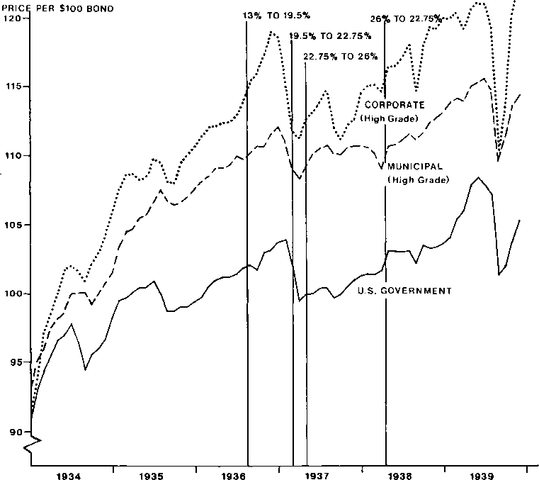
Figure 1. Monthly Prices of High-Grade Corporate, Municipal, and U.S. Government Bonds.

The second aspect of this question of the effectiveness of fiscal policy in the thirties deals not with crowding out, but with the effects on the structure of prices and resource allocations due to an increase in net aggregate spending resulting from expansionary fiscal policy.32 Suppose that the increase in federal government spending had been funded by an increase in the stock of money courtesy of an accommodating Federal Reserve System policy. In such a situation, nominal spending by the private and nonfederal government sectors would not have to decline. There is still reason to expect that this expansionary fiscal policy, now accommodated by an expansionary monetary policy, would not have more quickly brought about full employment.

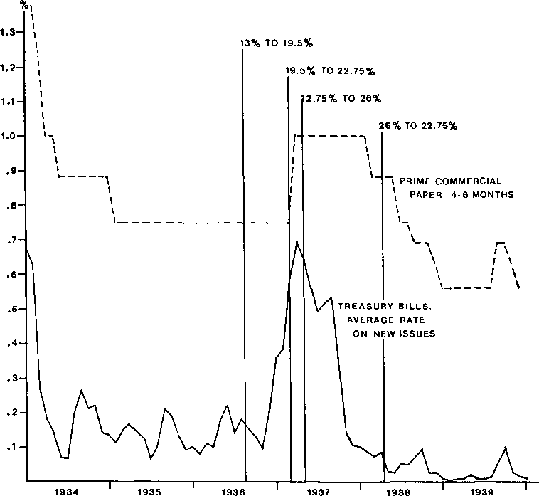
Figure 2. Prime Commercial Paper Rate and Average Rate on New Treasury Bills

Macroeconomic analysis generally does not distinguish between types of expenditures made by the federal government as it pursues expansionary fiscal policy. It does suggest that the multipliers may be somewhat larger or smaller for different types of expenditures since, with constant prices, fixed coefficients of production, and idle resources, some expenditures have larger backward linkages. All expenditures, however, are assumed to have positive multipliers and the amount of the increase in federal spending is generally considered much more important than the particular types of increased federal expenditures.

The evidence, however, does not indicate that these conditions existed. Not only was there a severe price deflation during the Depression and a price inflation from 1933 on, but there were pronounced changes in relative prices during the thirties.33 In addition, federal expenditures often have pronounced local effects which are much more important in magnitude and timing than any general economywide effects arising from the operation of the multiplier.34

To explain why an increase in federal spending in excess of spending declines in other sectors may well not have promoted recovery, it is useful to briefly review the role of relative prices in a market economy.35 Austrians define an “equilibrium” as a situation where the plans of each and every transactor are mutually consistent. In his writings, Friedrich Hayek argued that we should speak of the tendency for mutually compatible plans to come about rather than speak of actually achieving equilibrium. With respect to this, Hayek suggested that the “division of knowledge” was at least as important as the division of labor, yet it had been completely neglected.

The problem which we pretend to solve is how the spontaneous interaction of a number of people, each possessive only bits of knowledge, brings about a state of affairs in which prices correspond to costs, etc., and which could be brought about by deliberate direction only by somebody who possessed the combined knowledge of all those individuals.36

The mechanism that tends to bring the plans of individual transactors into closer correspondence with each other is the price system. Hayek proposed that people consider the price system as a mechanism for economically transmitting information among transactors. It is this mechanism that has to be the focus of any study of the coordination problem that all economic systems face. Gerald P. O’Driscoll describes this as follows:

The price system registers both the effects of changing objective conditions and the reactions of transactors to these changes. Most important, the price system is a mechanism—however imprecise—for registering the ever-changing expectations of market participants. What is important here is the argument that the price system is the cheapest possible system of resource allocation.37

When there are cyclical fluctuations, such as the Great Depression of 1929–33, Austrians focus on the coordination problem to explain and understand why there is a breakdown in a market system—a system that is supposed to work and previously had been working. In a cyclical contraction, discoordination of markets leads to declines in production and incomes as well as increases in idled resources (labor and capital). Relative prices are the primary economic data providing the information tending to coordinate the plans of individual transactors. To understand and explain the contraction, economists must search for the forces that alter relative prices in ways that provide incorrect information that tends to discoordinate market behavior. The recovery phase of the cycle consists of discovering and establishing the relative prices that tend to coordinate the plans of the individual transactors, and that complete the resource reallocations begun during the contraction phase of the cycle.

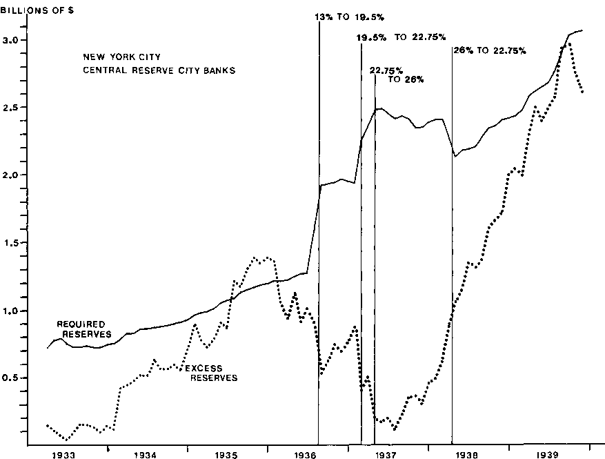
Figure 3. New York City, Central Reserve City Banks

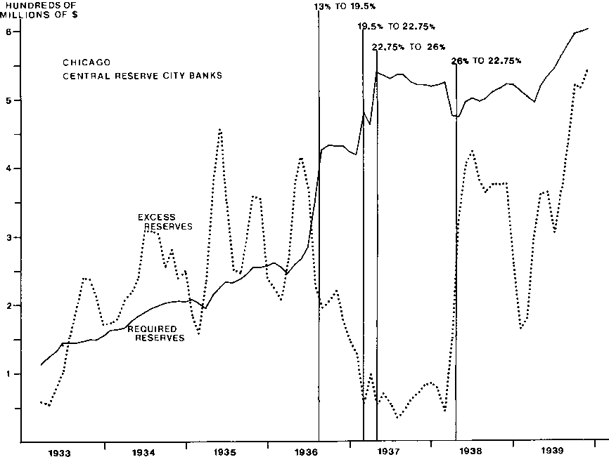
Figure 4. Chicago, Central Reserve City Banks

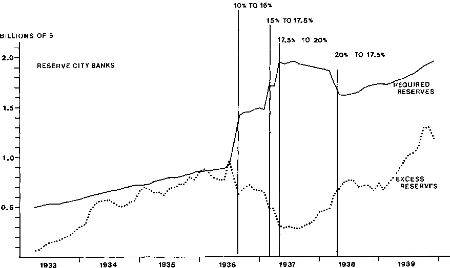
Figure 5. Reserve City Banks

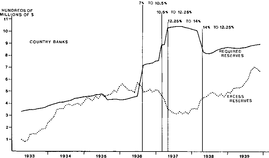
Figure 6. Country Banks

Several Austrian economists have examined the Great Depression. I can draw upon their analyses here.38 Austrians point out that business cycles are “monetary disturbances [which] alter the array of relative prices by affecting market interest rates and the pattern of investment.”39 During the 1920s, the expansion of the stock of money through the banking system caused interest rates to be lower than they otherwise would have been. This inflation led to “malinvestments” as the lower discount rates induced entrepreneurs to shift productive resources toward uses further removed in time from final consumption. Since consumer preferences had not actually shifted toward future consumption, once the rate of growth of the money stock failed to increase or even slowed down, interest rates began rising and the recent investments in resources further removed from consumption proved not to be profitable.40

Lionel Robbins, Friedrich Hayek, and Murray Rothbard particularly blamed the Federal Reserve System’s easy money policy in the last half of 1927 for leading into a more severe contraction than otherwise would have been necessary. Hayek said that until 1927, he would have expected a mild depression since in the preceding boom period, prices did not rise. However, the Federal Reserve System’s expansion of the stock of money beginning in mid-1927 prolonged the boom for two more years and made the Depression more severe.41

When the inflationary expansion of the stock of money ceased at the end of 1928, the Depression was inevitable. Production indices began declining in the second quarter, stock market transactors recognized what was happening, and stock prices ceased rising at the end of the third quarter, and the stock market “crashed” at the end of October 1929. The “overinvestments” discovered by later analysts were not the general overinvestments, but rather the malinvestments of the boom which were shown to be unprofitable once the money growth stopped.

Murray Rothbard has made a detailed examination of the Hoover administration’s actions which lengthened the Depression and made it much more severe.42 In November 1929, Hoover met with the leaders of the major industrial firms, the heads of the leading public utilities, representatives of the building and construction industry, and leading labor union officials. He asked that money wages not be cut (to maintain purchasing power) and, when necessary, the workweek be reduced as an alternative to layoffs. These leaders were receptive to his requests. Money wage rates in twenty-five major industries remained constant until late 1930. Many businesses resisted wage rate cuts until quite late in 1931. U.S. Steel, over the opposition of its president, finally cut wage rates in September 1931. Other firms cut wages secretly “for fear of the disapproval of the Hoover Administration.”43

This policy led to much greater declines in output and employment since holding money wage rates constant raised real wage rates as prices fell. In fact, real wage rates in June 1933 were higher than in June 1929. The primary problem was not that the policy did not allow wage rates to fall since not all wage rates had to decline. Rather, it did not allow the wage rates for the various occupations and for the various firms to adjust as necessary to coordinate labor and other markets.

The Hawley-Smoot Tariff was approved and put into effect in June 1930. The protective tariff raised rates to the highest in U.S. history and spawned retaliatory tariffs in many other nations. This set off a spiraling contraction of both U.S. imports and exports, and altered the demands and supplies of many products and services requiring substantial relative price adjustment and resource movements.

The Federal Farm Board, established in 1929, attempted to support the prices of wheat and many other farm products. Production rose, surpluses piled up, and world prices continued to fall. Finally the FFB began dumping its surplus holdings on world markets, driving down prices and further undermining the farmers’ positions.

In 1932, Congress approved huge increases in tax rates for most federal taxes. The sharp decline in the stock of money (which began in 1931 and accelerated in late 1931, after Great Britain went off gold) continued. The Reconstruction Finance Corporation, created in 1932, made a number of loans to ailing banks. Publication of these loans led to runs on these banks as the public interpreted the loans as a sign of weakness. This, combined with the worry that Roosevelt would devalue gold (or take the United States off the gold standard), led to massive and continued bank runs by the end of 1932. With these runs there were, for the first time, specific demands for gold.

The deflationary decline in the money stock and the intermittent banking panics required further relative and absolute price adjustments. The reductions in bank lending required that interest rates be higher than they otherwise would have been. Prices of financial assets, productive resources, and goods and services had to fall in complex sequential patterns. The result was a highly complex alteration of relative prices while the declining money stock caused prices to fall.44

By the trough of the Depression, these shocks to the economy and the discoordination of various markets (particularly the labor markets) required large resource shifts and relative price changes to bring about higher employment and output levels. The process of recovery required these price changes and resource shifts.

This was and, of course, still is no simple task. With price searching firms, each firm has to discover each resource and product price through a trial and error process of trying different prices—a search process that can be long and difficult. In a dynamic environment, there is no simple and direct path from the prevailing disequilibrium price toward a new price consistent with all other prices.

This process is not part of the logic behind fiscal policy. The Keynesian approach simply asserts that what is necessary is to obtain a net increase in aggregate spending. Since the federal government’s spending is not constrained by income, wealth, cash flows, or profitability, then it is up to the federal government to initiate the spending increase. The general logic of the Keynesian model does not suggest that it makes any important difference what type of federal spending is increased.

When one recognizes that the problem is one of price and resource adjustments to coordinate the plans of consumers and firms, fiscal policy’s impact changes. It will not initiate a more rapid recovery unless the federal expenditures promote coordinating price adjustments. This, however, was as unlikely then as now. The knowledge of how relative prices should be altered to promote the appropriate resource adjustments is not something that any individual or group(s) of individuals in the government or elsewhere has. As Hayek has pointed out, it is dispersed among all of the participants in the economy.

The fiscal policies of the federal government during the recovery included a number of tax increases as well as increased spending. Much of the increased spending was on make-work jobs to give employment to those who were unemployed rather than simply provide direct relief funds, though there also was much direct relief. I can briefly note some of the projects on which the federal government increased its spending.45 The Public Works Administration undertook a number of large-scale projects such as highway, dam, and large public building construction as well as harbor improvements. The Civil Works Administration undertook “new and improved roads; bridges; repair of 40,000 schools; drainage of hundreds of thousands of acres of malarial lands; destruction of millions of rats and ticks; 150,000 sanitary privies; 200 swimming pools; 3,700 playgrounds; new hospitals; athletic stadiums; airports; and public buildings.” The Civil Works Service Program employed “nonmanual labor” on many cultural projects such as paintings, sculptures, murals, writing music, and compiling local histories. The Emergency Education Program provided work for unemployed teachers in “adult education, vocational education and rehabilitation, and nursery schools for underprivileged children.” The Women’s Work Program provided “homemaking” type jobs for women in such activities as “sewing clothes, making bedding, canning food, nursing, teaching, research, and making statistical surveys.”46 The Civilian Conservation Corps sent young people off to camps, especially in forests and national parks, to do conservation work.

These types of projects were continued in the Works Progress Administration. The WPA constructed streets, sidewalks, water supply systems, sewage disposal systems, parks, airports, public buildings, hospitals, penal institutions, and military establishments. It sealed mines; undertook water conservation projects and engineering surveys; set up nursery schools; provided library services; sponsored adult education, museum, music, writing, art, and theater projects; provided social, economic, housing, and national health surveys; and organized a number of other welfare projects.47

The Reconstruction Finance Corporation provided loans and purchased stock to prop up financial institutions. Agricultural credit was provided to farmers and the Agricultural Adjustment Administration spent funds to raise farm prices and limit farm production.

There is no evidence that these types of expenditures promoted coordination of the plans and actions of individuals and firms. Many of these projects involved “public” or conservation projects which would not have been undertaken otherwise and which were not the type that private enterprise would have undertaken. Offsetting the coordination that these federal expenditures brought about were other aspects of these and other New Deal programs.

At the time, it was noted that the labor required for many of the public works projects (such as roads, buildings, and bridges) “could not provide appropriate employment for many types of the unemployed.”48 Wage and hours policies also were controversial. There was considerable discussion of whether the wages should be at the prevailing level or lower than prevailing wages to encourage workers to seek employment in private industry. The general policy was to pay the prevailing wage rates “except where these were below the stated minimum levels” and to establish maximum hours of work.49 Minimum wage rates and maximum hours of employment per week were written into a number of New Deal laws. Such actions certainly did not facilitate the market adjustments necessary to coordinate markets, particularly the labor markets.

Other New Deal programs severely hindered market processes. The NIRA’s attempt to cartelize much of U.S. business virtually stopped the recovery. In attempting to stop price competition and raise prices, it tried to control and set uniform prices, raise and equalize wage rates, eliminate nonprice as well as price competition, and stop investment if there were any excess capacity in other firms in the industry.50 The promotion of unionization following the Wagner Act, the late 1930s antitrust crusade, and the creation of an unending agricultural crisis through price support programs all made the coordination of markets much more difficult. By reducing the ability of prices to adjust in response to changes in market conditions, it became more difficult to bring about greater consistency in the plans of the market participants. These New Deal programs—combined with federal expenditures concentrated on producing public and cultural works and the construction of public buildings and other capital goods—lengthened the recovery from the Great Depression.

On the basis of this analysis, I conclude that the evidence indicates that a more expansionary fiscal policy would not have brought about a faster recovery from the Great Depression. First, the evidence suggests that an expansion of federal spending, financed by the sale of U.S. government securities rather than by tax increases and without the Federal Reserve System “monetizing” the additional federal debt, would have, for all practical purposes, have been offset by induced decreases in private and nonfederal government spending. Second, there is no reason to think that increases in net aggregate spending initiated by increased federal spending would have been likely to alter relative prices in ways that would have promoted coordinating adjustments toward higher employment and output. This would not have been an objective in the decision as to how the expenditures should have been undertaken. Even if the increased federal spending had been accommodated by an expansionary monetary policy, there is a low likelihood that the pattern of spending would have been such as to promote equilibrating price adjustments. Previous analyses of Keynesian fiscal policy in the recovery from the Great Depression have failed to adequately examine either crowding out effects or effects on the structure of relative prices, and, therefore, were misleading as to the potential effects of expansionary fiscal policy.

Appendix: The Early 1940s Recovery

One of the reasons that Keynesian analysis became widely accepted and still has many adherents is the belief that the early 1940s proved that Keynesian expansionary fiscal policy “worked” in promoting a more rapid return to full employment. From 1940 on, the federal government rapidly expanded its spending under the impetus of preparation for and then involvement in World War II. Most economic history and macroeconomics textbooks still single out this period as evidence of the power of Keynesian fiscal policy.

This acceptance is primarily a matter of faith rather than analysis. The early 1940s recovery cannot be seen as evidence that pure Keynesian fiscal policy works since, to give just one example, the Federal Reserve System authorities dramatically changed monetary policy. Under the pressures of the war in Europe and, presumably, the likely involvement of the United States, the Federal Reserve System adopted an extremely expansionary monetary policy at the start of 1940. From January 1940 through January 1941, the stock of money grew 12.01 percent, then 22.88 percent from January 1940 through January 1942, and 44.78 percent from January 1940 through January 1943. Through 1940 and 1941, nearly 90 percent of the growth of the stock of money was due to the growth of the high-powered money, controlled by the Federal Reserve System.51 The change in monetary policy, in effect, allowed a monetization of the debt the federal government issued as its spending rapidly increased. With such an expansionary (or inflationary) monetary policy, economists cannot conclude that it was fiscal policy rather than monetary policy that was the proximate cause of the more rapid recovery.

I have argued above that there is no reason to think that either fiscal policy with debt monetization or pure monetary policy would necessarily promote higher employment and output unless the additional expenditures tended to promote greater coordination of the plans of individual transactors through the appropriate relative price adjustments. There is, in fact, reason to believe that something such as this did occur. To understand why this is so, one needs to consider the unionization that occurred in the late 1930s.

Following the Wagner Labor Relations Act of 1935, there was an accelerated drive to unionize various firms—often all the firms in an industry. This was concentrated in the major industries containing the largest firms. For the most part, rather lengthy and bitter strikes were necessary to bring union recognition. Once the unions were recognized as the monopoly bargaining agents for the firm’s workers, relatively large wage rate increases were negotiated as well as reductions in working hours. For example, when U.S. Steel and many smaller steel firms were organized in 1937, wage rates rose 19 percent (from 52.5 to 62.5 cents an hour) and overtime wage rates were installed. “Little Steel” temporarily staved off unionization by granting the same wage increase. It appears that similar types of wage and hour agreements were concluded in most cases of successful unionization in the late 1930s.

There has been little analysis of the firms’ responses to these increased operating outlays. Yet, one would expect the magnitude of the wage rate changes to have noticeable effects. All else remaining the same, the increases in labor expenditures would cause the firms to discover some combination of higher prices for the products being produced as well as reduced production (because of the higher product prices). Employment in the newly unionized firms would decline because of the reduced production and because firms would begin the process of marginally substituting capital for labor due to the higher relative price of labor.

If the demands for the products of the newly unionized firms were increasing, then their product prices might not have to rise and production might not decline. In time, there would still be some reduction in employment due to the marginal substitution of capital for labor. The problem is that we do not know what the conditions were in the late 1930s. No examination of the responses of the various firms seems to have been undertaken. There are no data on product prices, labor costs, employment, and production for both the firms that underwent unionization and those that did not.

My guess is that there were no relative increases in demand for the firms being unionized. If this were the case, then those firms had to choose some combination of increased product prices and relatively reduced production and employment. This would seem likely because of the 1937–38 contraction and the slow recovery from mid-1938 to 1940, as well as the fact that there is no reason to think that the demands for the products of the unionized firms would have been growing faster than the demands for the products of firms not being unionized.52 This would have slowed down the recovery. Workers who were employed and would have been employed by these firms would thus have had to search for employment elsewhere. Most of the firms being unionized were large, heavy industry firms and their plants dominated the communities in which they were located. It is likely that workers would have had to extend their search toward other locations to discover employment opportunities. Since the products of some of the unionized firms were inputs into final products of other firms, there would be a complex alteration of the relative prices and production of many other products. Thus, the process of firms discovering whether the demand for their output had increased or decreased (and whether this was temporary or permanent), as well as workers discovering where employment opportunities were and what were the employment conditions, would have slowed the movements toward higher employment and production.

The federal government’s expenditures on war goods in 1940, 1941, and 1942 tended to be concentrated on materials produced by heavy industry firms, firms where the late 1930s unionization had been concentrated. The result was that federal expenditures on war materials largely tended to increase demands in those industries where it is likely that costs had increased without commensurate demand increases in the late 1930s. This would have allowed them to profitably expand employment and production. The federal government’s war expenditures at the beginning of the 1940s, financed largely by an increasing stock of money, are likely to have unintentionally promoted a number of equilibrating price and resource adjustments. The increased coordination would have more rapidly increased employment and output.53

The empirical research necessary to address the question of why there was such a rapid recovery in the early 1940s has not yet been undertaken. It should be noted that the question is not one of theory; rather it is one of empirical facts.54 What were the demand conditions in the late 1930s and early 1940s for firms that were unionized and those that were not? How did the managements of the unionized firms respond to these changes? To what firms did the federal government’s early 1940s war purchases go, and in what magnitudes? This constitutes an important empirical research agenda. What is presently clear is that the rapid recovery of the early 1940s is neither evidence nor proof that Keynesian fiscal policy “works” nor evidence that it would have restored full employment much more rapidly in the 1933–39 period.

References

Arrington, Leonard J., (1969), “The New Deal in the West: A Preliminary Statistical Inquiry.” Pacific Historical Review 38, 311–16.

———, (1970), “Western Agriculture and the New Deal.” Agricultural History 44, 337–53.

Bailey, Martin J. (1962, 1971), National Income and the Price Level. New York: McGraw-Hill.

Barro, Robert J. (1974). “Are Government Bonds Net Wealth?” Journal of Political Economy 82, 1095–1117.

Bernanke, Ben S. (1983), “Nonmonetary Effects of the Financial Crisis in the Propagation of the Great Depression.” American Economic Review 73, 257–76.

Beveridge, W.H. (1930), Unemployment: A Problem of Industry. London: Longmans, Green.

———, (1931), Causes and Cures of Unemployment. London: Longmans, Green.

Board of Governors of the Federal Reserve System (1943), Banking and Monetary Statistics. Washington, D.C.: National Capital Press.

Boorman, John T. (1980), “The Evidence on the Demand for Money: Theoretical Formulations and Empirical Results,” pp. 315–60 in Thomas M. Havrilesky and John T. Boorman, eds., Current Issues in Monetary Theory and Policy, 2nd ed. Arlington Heights, Ill.: AHM Publishing.

Brown, E. Cary (1956), “Fiscal Policy in the Thirties: A Reappraisal.” American Economic Review 46, 857–79.

Brunner, Karl, ed. (1981), The Great Depression Revisited. Boston: Martinus Nijhoff.

Chandler, Lester V. (1970), America’s Greatest Depression, 1929–1941. New York: Harper & Row.

Conkin, Paul P. (1975), The New Deal, 2nd ed. Arlington Heights, Ill.: AHM Publishing.

Darby, Michael R. (1976), “Three-and-a-Half Million U.S. Employees Have Been Mislaid: Or, an Explanation of Unemployment, 1934–1941.” Journal of Political Economy 84, 1–16.

Dolan, Edwin G., ed. (1976), The Foundations of Modern Austrian Economics. Kansas City: Sheed and Ward.

Dublin, Louis (1943), A Family of Thirty Million: The Story of the Metropolitan Life Insurance Company. New York: Metropolitan Life Insurance.

Friedman, Milton, and Anna Schwartz (1963), A Monetary History of the United States: 1867–1960. Princeton: Princeton University Press.

Gallaway, Lowell, and Richard Vedder (1985), “Wages, Prices, and Employment: Von Mises and the ‘Progressives’.” Manuscript, Ohio University, 1985.

Gandolfi, Arthur E. (1974), “Stability of the Demand for Money during the Great Contraction—1929–1933.” Journal of Political Economy 82, 969–84.

Gandolfi, Arthur E. and James R. Lothian (1976), “The Demand for Money from the Great Depression to the Present.” American Economic Review 66, 46–51.

Garrison, Roger (1978), “Austrian Macroeconomics: A Diagrammatical Exposition,” pp. 167–204 in Louis M. Spadaro, ed., New Directions in Austrian Economics. Kansas City: Sheed and Ward, 1978.

Havrilesky, Thomas M., and John T. Boorman, eds., (1980), Current Issues in Monetary Theory and Policy, 2nd ed. Arlington Heights, Ill.: AHM Publishing.

Hawley, Ellis W. (1965), The New Deal and the Problem of Monopoly, 1933–1939. Princeton: Princeton University Press.

Hayek, Friedrich A. (1931, 1967), Prices and Production. New York: Augustus M. Kelly.

———, (1933), Monetary Theory and the Trade Cycle. London: Jonathan Cape.

———, (1948), Individualism and Economic Order. Chicago: Henry Regnery, a Gateway edition.

———, (1979), Unemployment and Monetary Policy: Government as Generator of the “Business Cycle,” Paper no. 3. San Francisco: Cato Institute.

Hickman, Bert, and Robert Coen (1976), An Annual Growth Model of the U.S. Economy. Amsterdam: North-Holland.

Hughes, Jonathan R.T. (1977), The Governmental Habit: Economic Controls from Colonial Times to the Present. New York: Basic Books.

———, (1983), American Economic History. Glenview, Ill.: Scott, Foresman.

Kesselman, J.R., and N.E. Savin (1978), “Three-and-a-Half Million Workers Never Were Lost.” Economic Inquiry 16, 205–25.

Khan, Mohsin S. (1974), “The Stability of the Demand-for-Money Function in the United States 1901–1965.” Journal of Political Economy 82, 1205–19.

Kimmel, Lewis H. (1939), The Availability of Bank Credit, 1933–1938. New York: National Industrial Conference Board.

Kindleberger, Charles P. (1973), The World in Depression, 1929–1939. Berkeley: University of California Press.

King, Wilford I. (1938), The Causes of Economic Fluctuations. New York: Ronald Press Co.

Kirzner, Israel M. (1973), Competition and Entrepreneurship. Chicago: University of Chicago Press.

———, ed. (1982), Method, Process, and Austrian Economics: Essays in Honor of Ludwig von Mises. Lexington, Mass.: Lexington Books.

Klebaner, Benjamin (1974), Commercial Banking in the United States: A History. Hinsdale, Ill.: Dryden.

Kormendi, Roger C. (1983), “Government Debt, Government Spending, and Private Sector Behavior.” American Economic Review 73, 994–1010.

Lachmann, Ludwig M. (1976), “Toward A Critique of Macroeconomics,” pp. 152–59 in Edwin G. Dolan, Ed., The Foundations of Modern Austrian Economics. Kansas City: Sheed and Ward, 1976.

Laidler, David E.W. (1969), The Demand for Money: Theories and Evidence. Scranton, Pa.: International Textbook.

Lebergott, Stanley (1984), The Americans: An Economic Record. New York: W.W. Norton.

Leuchtenberg, William E. (1963), Franklin D. Roosevelt and the New Deal. New York: Harper & Row.

Lyon, LeVerett S., et al. (1935), The National Recovery Administration: An Analysis and Appraisal. Washington, D.C.: The Brookings Institution.

Mitchell, Broadus (1947), Depression Decade: From New Era Through New Deal, 1929-1941. New York: Rinehart.

Mises, Ludwig von (1966), Human Action: A Treatise on Economics, 3rd rev. ed. Chicago: Henry Regnery.

Nash, Gerald D. (1979), The Great Depression and World War II: Organizing America, 1933–1945. New York: St. Martin’s.

O’Driscoll, Gerald P., Jr., (1977) Economics as a Coordination Problem: The Contributions of Friedrich A. Hayek. Kansas City: Sheed, Andrews, and McMeel.

———, (1978), “Spontaneous Order and the Coordination of Economic Activities,” pp. 111–42 in Louis M. Spadaro, ed., New Directions in Austrian Economics. Kansas City: Sheed and Ward, 1978.

O’Driscoll, Gerald P., Jr. and Sudha R. Shenoy (1976), “Inflation, Recession, and Stagflation,” pp. 185–211 in Edwin G. Dolan, ed., the Foundations of Modern Austrian Economics. Kansas City: Sheed and Ward, 1976.

Peppers, Larry C. (1973), “Full-Employment Surplus Analysis and Structural Change: The 1930’s.” Explorations in Economic History 10, 197–210.

Reading, Don C. (1973), “New Deal Activity and the States, 1933 to 1939.” Journal of Economic History 33, 792–810.

Rizzo, Mario J., ed. (1979), Time, Uncertainty, and Disequilibrium: Explorations of Austrian Themes. Lexington, Mass.: Lexington Books.

Robbins, Lionel (1934), The Great Depression. New York: Macmillan.

Rockoff, Hugh (1984), Drastic Measures: A History of Wage and Price Controls in the United States. New York: Cambridge University Press.

Rothbard, Murray N. (1962, 1970), Man, Economy and State: A Treatise on Economics, 2 vols. Los Angeles: Nash.

———, (1963), America’s Great Depression. Kansas City: Sheed and Ward.

Schlesinger, Arthur M., Jr. (1957–60), The Age of Roosevelt, 3 vols. Boston: Houghton Mifflin.

Schumpeter, Joseph A. (1939), Business Cycles, 2 vols. New York: McGraw-Hill.

Smiley, Gene (1981), “Regional Variation in Bank Loans Rates in the Interwar Years.” Journal of Economic History 41, 899–901.

Spadaro, Louis M., (1978), New Directions in Austrian Economics. Kansas City: Sheed and Ward.

Stein, Herbert (1969), The Fiscal Revolution in America. Chicago: University of Chicago Press.

Stoddard, W.L. (1940), “Small Business Wants Capital.” Harvard Business Review 18, 265–74.

U.S. Dept. of Commerce, Bureau of the Census (1976), Historical Statistics of the United States: Colonial Times to 1970. Washington, D.C. U.S. GPO.

U.S. National Resources Planning Board (1942), Security, Work, and Relief Policies. Washington, D.C.: U.S. GPO.

Viner, Jacob (1935), Balanced Deflation, Inflation, or More Depression? Minneapolis: University of Minnesota Press.

Weinstein, Michael M. (1980), Recovery and Redistribution under the NIRA. Amsterdam: North-Holland.

———, (1981), “Some Macroeconomic Impacts of the National Industrial Recovery Act, 1933–1935,” chap. 14 in Karl Brunner, ed., The Great Depression Revisited. Boston: Martinus Nijhoff.

Williamson, Harold G., and Orange A. Smalley (1957), Northwestern Mutual Life: A Century of Trusteeship. Evanston, Ill.: Northwestern University Press.

Wright, Gavin (1974), “The Political Economy of New Deal Spending: An Econometric Analysis.” Review of Economics and Statistics 56, 30–38.

Substantial portions of this study were undertaken while I was a fellow at the Liberty Fund-Institute of Humane Studies 1983 summer research seminar on historical aspects of political power and individual freedom. Useful comments were provided by all of the participants as well as colleagues at Marquette University, but I wish to especially acknowledge the comments of Steven Crane, Lowell Gallaway, Thomas Humphrey, Paul McGouldrick, Murray Rothbard, Sudha Shenoy, Richard Timberlake, Richard Vedder, and several anonymous referees. All errors and omissions are, of course, my responsibility.

Gavin Wright later reexamined the issue, arguing that the political factor had to be taken into account. Wright’s study convincingly argued that New Deal spending tended to be concentrated in those states where the spending was more likely to change the course of an election because the voting was expected to be close or there had been substantial swings in voter sentiment in the past. This brings into question one of the most fundamental assumptions of Keynesian macroeconomic analysis. See Gavin Wright, “The Political Economy of New Deal Spending: An Econometric Analysis,” Review of Economics and Statistics 56 (February 1974), pp. 30–38.

• 1Historical Statistics of the United States, part 1 (Washington, D.C.: 1975), series D-86 for unemployment rates and series F-32 for gross national product. Throughout this article, the standard data series for unemployment rates are used, with recognition that there has been a challenge to the validity of those data during the Great Depression years. See Michael R. Darby, “Three-and-a-Half Million U.S. Employees Have been Mislaid: Or An Explanation of Unemployment, 1934–1941,” Journal of Political Economy 84, 1976.
• 2A.C. Pigou, Industrial Fluctuations, 1st ed. (London: Macmillan, 1927), p. 176.
• 3A.C. Pigou, Theory of Unemployment (London: Macmillan, 1933), p. 252. Pigou makes his arguments in a variety of other places. For example, see his “Real and Money Wage Rates in Relation to Unemployment,” Economic Journal 47, 1937, and “Money Wages in Relation to Unemployment,” Economic Journal 48, 1938.
• 4It is perhaps something of an exaggeration to ascribe this position entirely to Pigou. A number of other economists espoused similar views. Recognizing that the list is incomplete, we cite a few, beginning with Jacob Viner, Balanced Deflation, Inflation, or more Depression (Minneapolis, Minn.: University of Minnesota Press, 1933), especially pp. 12–13. See also W.H. Beveridge, Causes and Cures of Unemployment (London: Longmans, Green and Co., 1931), p. 25, and Unemployment, A Problem of Industry (London: Longmans, Green and Co., 1930), chapter 16; Wilford I. King, The Causes of Economic Fluctuations (New York: Ronald Press Co., 1938), chapter 8; and Lionel Robbins, The Great Depression (New York: Macmillan, 1934).
• 5John A. Hobson, The Economics of Unemployment (New York: Macmillan, 1923), p. 84.
• 6W.T. Foster and W. Catchings, Profits (Boston: Houghton Mifflin, 1925) and Business Without a Buyer (Boston: Houghton Mifflin, 1927); and C.H. Douglas, Credit-Power and Democracy (London: C. Palmer, 1920) and Warning Democracy (London: C.M. Grieve, 1931). A more recent interpretation of the Great Depression with underconsumptionist overtones in John Kenneth Galbraith, The Great Crash, 1929 (Boston: Houghton Mifflin, 1976).
• 7Murray N. Rothbard, America’s Great Depression (Princeton, N.J.: Van Nostrand, 1963), p. 45.
• 8Henry Ford, The New York Times, November 22, 1929, p. 2.
• 9The New York Times, November 22, 1929, p. 1. It is interesting to note that Hoover’s inclinations toward underconsumptionism were recognized and, of course, approved, by trade unionists. Witness a statement by the AFL’s John P. Frey in 1929 relating to a public works scheme of Hoover’s. In effect, Frey argued that the president was in agreement with the AFL’s position that depressions were the result of underconsumption and low wages. See Joseph Dorfman, The Economic Mind in American Civilization (New York: Viking Press, 1959), vol. 4, pp. 349–50. See also Ronald Radosh, “The Development of the Corporate Ideology of American Labor Leaders, 1914–1933” (doctoral dissertation in history, University of Wisconsin, 1967).
• 10Rothbard, America’s Great Depression, chapter 8. Not to be ignored is the fact that ideas such as those that enamored Hoover were not as unorthodox among professional economists as sometimes claimed. See J. Ronnie Davis, The New Economists and the Old Economists (Ames, Iowa: Iowa State University Press, 1971). Davis presents an interesting array of statements by economists and other academics relating to the issue of the impact of wage reductions on the economy (pp. 94–99).
• 11John M. Keynes, The General Theory of Employment, Interest and Money (London: Macmillan, 1936).
• 12Abba P. Lerner, “Mr. Keynes’ ‘General Theory of Employment, Interest and Money,’” International Labor Review 34, 1936. See also W.B. Reddaway, “The General Theory of Employment, Interest and Money,” Economic Record 12, 1936. A systematic description of the thought of this time is contained in Lawrence R. Klein, The Keynesian Revolution (New York: Macmillan, 1947). For a taxonomic description of the various views of the aggregate demand schedule for labor, see Sidney Weintraub, “A Macroeconomic Approach to the Theory of Wages,” American Economic Review 46, 1956.
• 13Paul M. Sweezy, personal letter to John B. Shelley, dated February 11, 1977, cited in Dana C. Hewins and John B. Shelley, “Sweezy’s Kink: Macro Foundations of a Micro Theory,” Economic Inquiry 17, 1979.
• 14For a description of the various dimensions of the Keynesian critique of classical economics, see Alvin H. Hansen, A Guide to Keynes (New York: McGraw-Hill, 1953). More recent appraisals and restatements of the total thrust of Keynesianism are Abba P. Lerner, “From ‘The Treatise on Money’ to ‘The General Theory,’” Journal of Economic Literature 12, 1974; and Hyman P. Minsky, John Maynard Keynes (New York: Columbia University Press, 1975).
• 15Peter Temin, Did Monetary Forces Cause the Great Depression? (New York: Norton, 1976), p. 140. Temin also attempts to demonstrate that the Great Depression was brought on by an autonomous shift in the consumption function. That view has been challenged (successfully, we think) by Thomas Mayer, “Consumption in the Great Depression,” Journal of Political Economy 86, 1978.
• 16Keynes, The General Theory. In chapter 2, Keynes is very explicit. In reference to the principle that real wages and employment are systematically related, he says, “I am not disputing this vital fact which the classical economists have (rightly) asserted as indefeasible.”
• 17Ludwig von Mises, The Theory of Money and Credit (New Haven, Conn.: Yale University Press, 1953). Permission granted by Mrs. Margit von Mises. Quotes from 1981 Liberty Classics, Indianapolis, edition.
• 18Milton Friedman, “The Role of Monetary Policy,” American Economic Review 58, 1968.
• 19In particular, see Jerome Stein, Monetarist, Keynesian, and New Classical Economics (Cambridge, United Kingdom: B. Blackwell, 1982).
• 20The key assumptions are constant returns to scale and neutral disembodied technical progress.
• 21The underlying statistical models are moderately complex. They are described briefly in the statistical appendix. The logic and structure of the models are more fully developed in Lowell Gallaway and Richard Vedder, The “Natural” Rate of Unemployment, staff study, Subcommittee on Monetary and Fiscal Policy, Joint Economic Committee, Congress of the United States (Washington, D.C.: 1982).
• 22Federal Reserve Bulletin, various issues.
• 23Historical Statistics, series D-86.
• 24The productivity-adjusted real wage rate on a quarterly basis is calculated by dividing the manufacturing wage bill by the product of Federal Reserve Board (not the wage bill) and the index of average labor productivity (not total output) should be used. However, converting the wage bill and the index of industrial production to wage rate and productivity measures involves dividing both of them by the same quantity of labor (L). Since L appears in both the numerator and denominator of the expression for the adjusted real wage rate, it cancels out and can be ignored.
• 25As calculated from Historical Statistics, series D-688.
• 26Ibid,, series D-683 and D-688.
• 27Ibid., series D-724 and Paul A. David and Peter Solar, “A Bicentenary Contribution to the History of the Cost of Living in America” in Paul Uselding, ed., Research in Economic History, vol. 2 (Greenwich, Conn.: JAI Press, 1977), pp. 59–60.
• 28Broadus Mitchell, Depression Decade, vol. 9, The Economic History of the United States (New York: Rinehart, 1947), p. 84; and Arthur Schlesinger, Jr., The Age of Roosevelt: The Crisis of the Old Order, 1919–1933 (Boston: Houghton Mifflin, 1957), p. 249. Interestingly, though, some observers of the period disagree with this assessment. For example, Leo Wolman, Wages in Relation to Economic Recovery (Chicago: 1931) notes, “[I]t is indeed impossible to recall any past depression of similar intensity and duration in which the wages of prosperity were maintained as long as they have been during the depression of 1930–1931.” Similarly, Don Lescohier, “Working Conditions,” vol. 3, History of Labor in the United States, 1896–1932, John R. Commons and Associates, eds. (New York: Macmillan, 1935) states:
• 29Historic Statistics, series D-802, D-813, D-818, and D-824, respectively.
• 30Robbins, The Great Depression, p. 224.
• 31Geoffrey H. Moore, ed., Business Cycle Indicators, vol. 2, Basic Data on Cyclical Indicators (Princeton: Princeton University Press, 1961), p. 129.
• 32Benjamin M. Anderson, Economics and the Public Welfare (New York: Van Nostrand, 1949), p. 72.
• 33Historical Statistics, series D-839.
• 34Anderson, Economics, p. 220.
• 35Without the productivity adjustment, real wages in manufacturing (in 1923 prices) rose from 58.9 cents an hour in December 1929 to 62.5 cents an hour in December 1930. After that, they continued to rise to 66.3 cents an hour in January 1932. Wilford I. King, Causes of Fluctuations, pp. 182–83. See also Sol Shaviro, “Wages and Payroll in the Depression, 1929–1933” (unpublished M.A. essay, Columbia University, 1947).
• 36Milton Friedman and Anna J. Schwartz, A Monetary History of the United States, 1867–1960 (Princeton, N.J.: Princeton University Press, 1963).
• 37U.S. Bureau of the Census, National Income and Product Accounts of the United States, 1929–1976 (Washington, D.C., Department of Commerce, Bureau of Economic Analysis, 1981), p. 308.
• 38Moore, Business Cycle Indicators, p. 106.
• 39Harold Barger, Outlay and Income in the United States, 1921–1938 (New York: National Bureau of Economic Research, 1942), appendix B, table 28. A smaller profit decline is reported in a less comprehensive survey conducted by the Federal Reserve Bank of New York. See Irving Fisher, Booms and Depressions: Some First Principles (New York: Adelphi, 1932), p. 98.
• 40Robbins, The Great Depression, p. 205. The data were originally published in Commercial and Financial Chronicle.
• 41This is based on the Standard and Poor’s index, which fell 32.9 percent from September to November 1929. The second decline actually began in April 1930. A similar pattern is observed using the Dow-Jones index, which fell 39.7 percent from April to December 1930, compared to 37.0 percent from September to November 1929. The recovery in stock prices after November 1929 was robust; the April 1930 Dow-Jones index was the eleventh highest recorded in history, exceeded only in the first ten months of 1929. See Moore, Cyclical Indicators, pp. 108–9.
• 42Ben Bernanke, “Nonmonetary Effects of the Financial Crisis in the Propagation of the Great Depression,” American Economic Review, June 1983, p. 261.
• 43Ibid., p. 262.
• 44Federal debt declined about $700 million in both 1929 and 1930, but rose more than $600 million in 1931. See Historical Statistics, series Y-493.
• 45If one uses the consumer price index to measure price changes, real interest rates on bank loans in 1929 averaged about 6 percent, rising to about 7.7 percent in 1930, and to about 13 percent in 1931. This is based solely on current year price changes. A real interest rate model using weighted averages of past price changes would show a smaller rise. Interest rate data are based on Federal Reserve System reports. See Moore, Cyclical Indicators, p. 154.
• 46Historical Statistics, series F-54.
• 47Friedman and Schwartz, A Monetary History, table A-1, pp. 712–13.
• 48Ibid., table B-3, p. 803.
• 49Ibid. The deposit/currency ratio fell from 11.57 in October 1929, to 4.44 in March 1933, a decline of 7.13 points, with 3.87 points (54 percent) of that decline occurring between October 1930 and October 1931.
• 50Ibid., pp. 308–13.
• 51The price would fall to $750 only for a consol, a bond with no maturity. Short-term bonds would sell at a small discount from face value because the owner of the bond would receive the face value at maturity.
• 52Historic Statistics, series X-581.
• 53Capital accounts were $10,372 million. Ibid., series X-587.
• 54Most nominal interest rate series show little change in the early years of the Great Depression, and, indeed, many show some decline. This masks two phenomena, however. First, declining commodity prices during the period led to rising real interest rates over time. Second, most interest rate series report actual transactions, probably ignoring a growing number of customers who were crowded out because of sharply rising risk premiums. It is possible that interest rates demanded of some average potential borrower rose, even though actual interest rates reflected in transactions did not rise.