Review of Austrian Economics

The Great Depression of 1946

Richard K. Vedder and Lowell Gallaway

It seems inevitable that some Ph.D. student in economics some time soon will pick up a recent copy of the Economic Report of the President looking for a dissertation topic and learn that there was a Great Depression in 1946, a topic which he or she will then analyze using all the tools of modern economic analysis. The student will read that real gross national product in 1946 fell 19 percent, the largest single decrease in annual output in the century of recorded annual GNP data.1 He or she will also learn quickly that from 1944 to 1947, real output fell by 22.7 percent. Looking up population figures, the student will observe that per capita output actually declined by more than one-fourth in real terms over the three years of conversion from war to peace, and did not regain the pre-depression (1944) level until 1964.2

From all of this the student will no doubt conclude that the heretofore neglected Great Depression of 1946 was the worst cyclical downturn in modern American economic history, and that by some measures it had a greater disruptive impact on the American economy than the earlier, more celebrated Great Depression of 1929–41. For example, in the earlier downturn, real per capita GNP surpassed the 1929 peak levels within 12 years, compared with 20 years it took to surpass the 1944 peak after the 1946 depression. Moreover, while the 1929–33 downturn was quantitatively a bit larger (30 percent vs. 23 percent), no single year exhibited a decline of the magnitude of that witnessed in 1946.

If the student is typical of most economics students today, he or she will lack a historical perspective. Therefore, that individual no doubt will fail to observe that the Great Depression of 1946 has been worsening every decade. In 1960, when Historical Statistics of the United States, Colonial Times to 1957 was published, the reported decline in real GNP in 1946 was but 7.8 percent, and for the three years 1944–47 just 9.8 percent, hardly a great depression.3 When the next edition of Historical Statistics was published in 1975, however, the 1946 decline was a more robust 12 percent, and the total business cycle downturn (1944–47) saw a drop in real output of 14.2 percent.4

By 1981, when the Department of Commerce reported revised national income data, the 1946 drop had reached a truly “depressing” 14.7 percent, with the episodic decline reaching 17.4 percent.5 Five years later, in 1986, the 1946 depression truly earned the label of “great” when the latest revisions in statistics revealed the 19 percent drop discussed above. The Great Depression of 1946 seems to be getting constantly worse, and if current trends continue should soon pass the 1929 depression in magnitude by any criteria.

If our mythical student looks further in the Economic Report of the President, he or she will get even more puzzled and, perhaps, excited. The student will learn that the sharp decline in GNP occurred with unemployment rates below four percent, far below the normal peacetime rate in the twentieth century, either before or after the 1946 “depression.”

He or she will also learn that this relatively full employment was achieved despite an extraordinarily contractionary fiscal policy. The federal budget deficit on a national income accounts basis in 1944 was some $54.5 billion, equal to 25.8 percent of GNP. That would be the equivalent in 1990 (in relation to GNP) of a deficit of about $1,400 billion. By 1947, the federal budget was in surplus by $13.4 billion, or 5.7 percent of GNP. The equivalent today (in relation to GNP) would be well over a $300 billion surplus. Among other things, the government in pursuing this extraordinarily contractionary fiscal policy fired (or “released from employment”) roughly 20 percent of the total labor force. All of this had little impact on unemployment.

We know of no episode in American economic history that more keenly illustrates several insights from Austrian economics than the 1944–47 business-cycle experience. The ultimate irony is that the modern historical interpretation of that era suggests that it was a period that demonstrated the superiority of Keynesian economic doctrines. It was in this period that the death knell came to residual sentiments among the American economics profession that market coordination is the most appropriate and efficient means to assure reasonably “full” employment of productive resources. Politically, it was during this period that the federal government institutionalized Keynesian-style macroeconomic intervention with the Employment Act of 1946.

Despite the statistics cited above, conventional modern wisdom is that the transition from war to peace proceeded without a major downturn after World War II, and certainly there was no “depression.”6 Our subsequent discussion will show that interpretation is essentially correct. However, it is generally accepted that the smooth economic conversion resulted from “pent up” demand for consumer goods offsetting the reduction in defense spending. In other words, the Keynesian prescription that “demand creates its own supply” worked after World War II.

After studying this historical episode, we conclude the following:

(1) Conventional wisdom is correct on one thing: there was no depression in 1946, or anything resembling one.

(2) Accordingly, aggregate economic statistics need to be viewed with a skeptical eye, particularly in periods such as this where there are pronounced governmental interventions in markets.

(3) The failure of the nation to enter a depression after 1944, however, reflected not pent-up consumer demand so much as the dramatically ameliorative effects of changing relative prices on the macroeconomy.

(4) The smooth transition to peace was accomplished despite the existence of a fiscal policy that was the very antithesis of Keynesian economic prescriptions to deal with falling aggregate demand. The most dramatically contractionary fiscal policy in modern American history failed to materially alter the pace of economic activity.

(5) Keynesian economics triumphed in politics and among academic economists at the very time that empirical evidence was clearly exposing its explanatory weaknesses. The very empiricist-quantitative economists who rhetorically were selling the new economics of Keynes on the grounds that the evidence of the 1929–41 downturn showed the empirical bankruptcy of market-oriented economic doctrines were ignoring, perhaps deliberately, the 1944–47 empirical evidence that was devastating to the Keynesian paradigm.

(6) A market-Austrian interpretation of this historical episode is very much more in keeping with the evidence.

Statistics Do Lie

Some official Department of Commerce statistics on this historical episode as they were published in 1960, and as they were published in 1990, are included in table 1. Note that every single series has somewhat different numbers in 1990 than in 1960. Changes are comparatively minor for money GNP, the civilian unemployment rate, and civilian unemployment, but they are substantial for price changes as measured by the GNP price deflator and, as a consequence, for real GNP. Table 2 summarizes the percent change in the five statistics over the 1944–47 period.

Between 1960 and 1990, government economists approximately doubled their estimate of the inflation occurring from 1944 to 1947, thereby causing the estimated real GNP decline to more than double.

Table 1
Some Key Economic Indicators as Reported in 1960 and in 1990
	Data Reported in 1960		Data Reported in 1990
Indicator	1944	1947	1944	1947
Civilian Unemployment Rate	1.2%	3.6%	1.2%	3.9%
Civilian Unemployment	670a	2,142a	670a	2,311a
GNP Price Deflator	115b	141b	15.3c	22.1c
Money GNP	$211.4d	$234.9d	$211.4d	$235.3d
Real GNP	$183.6b	$165.6b	$1,380.6c	$1,066.7c

aIn thousands

b1929 dollars

c1982 dollars

dIn billions

Sources: 1960 Data: Historical Statistics of the United States, Colonial Times to 1957; 1990 Data: Economic Report of the President, 1990.

Table 2
Percent Changes in Key U. S. Economic Indicators, 1944–1947
Indicator	1960 Data	1990 Data
Civilian Unemployment Rate	+200.0%	+225.0%
Civilian Unemployment (No.)	+219.7%	+244.9%
GNP Price Deflator	22.6%	44.4%
Money GNP	11.1%	11.3%
Real GNP	-9.0%	-22.7%

Source: Calculated from data found in table 1 above.

Substantial price controls were in effect in 1944, but were essentially abandoned by 1947. Thus official statistics based on controlled prices should tend to understate true equilibrium prices in 1944, and overstate the true inflation at market-clearing prices observed between 1944 and 1947. Yet the statistical revisions have tended to increase the reported inflation from 1944 to 1947, not decrease it. Following from that, the revisions in statistics over time have reduced the reported inflation during World World II. For example, reading the 1990 Economic Report of the President, one learns that the GNP price deflator rose a modest 13.8 percent in the four years 1941 to 1945, a lower annual rate of inflation than prevalent in the past two decades.7 Yet if one looks at, say, the 1978 Economic Report, the reported 1941–45 inflation is 20.3 percent.8 A few years earlier, in the 1975 edition of Historical Statistics, the wartime inflation was 26.5 percent.9 Picking up the 1960 version of Historical Statistics, however, the increase in prices was reported to be 29.7 percent.10 As time passes, it looks like the government was increasingly successful in curtailing inflation in World War II, and increasingly unsuccessful in containing it in the postwar era.

To this point, the various data revisions certainly seem to give justification to a common Austrian suspicion of over-reliance on aggregate economic statistics, particularly price indices, in evaluating the economy. Beyond that, the revisions serve to increase reported economic growth during the command economy era of World War II, and reduce it during the era in which there was a return to increased reliance on market forces in resource allocation, a conclusion that Austrians find hard to accept with equanimity.

Despite our suspicions to the contrary, we must concede, however, that it is possible that the earlier statistics were flawed, and that the revisions have served to paint a more accurate portrayal of the economic history of the period. Perhaps even there really was a major depression in 1946 that no one was perceptive enough to recognize at the time.

One way to evaluate that possibility is to try to ascertain what prices would have been in the 1942–48 period if various historical relationships observed earlier held. Using those forecasted or predicted prices, we can then estimate trends in real GNP using the money GNP statistics on which there has been virtually no data revision and little dispute (see, however, below).

We developed a model to predict the GNP price deflator for the period 1916 to 1941, the era immediately before the World War II experience where price controls were imposed. The years chosen were dictated largely by data considerations. Four independent variables were chosen, two financial in nature and two proxying for real output. The financial variables were M2 and the interest rate on four- to six-month commercial paper; the “real variables” were ton-miles of class A railroad volume and the total number of employed workers.11

Ordinary least squares regression procedures were used to estimate the GNP price deflator during the 1916–41 period. Actual values for the four independent variables were used with the estimated regression coefficients and constant term to calculate a forecasted value of the GNP price deflator for 1942 to 1948. The forecasting was aided by the fact that the estimated regression had a relatively good statistical fit (R2 = .822), with actual and estimated values being rather close for the years immediately preceding the war. (See the appendix for more details.)

Taking the estimated GNP price deflator numbers for 1942–48, along with the accepted money GNP numbers, we calculated real GNP by year. In table 3, we present our estimates, along with the official estimates as they were reported in 1960 and 1990. Turning first to prices, we estimated that true equilibrium prices rose far more during World War II than any of the official estimates. Our estimate is that prices rose 46 percent from 1941 to 1945, compared with official estimates varying, over time, between 24 and 30 percent. The historical experience from which our calculations were extrapolated was an era largely (although not completely) free of price controls. Our estimated price index thus incorporates the disguised inflation hidden by the existence of controls that was manifested in shortages, black markets, shoddy quality of goods or services, etc.12

Table 3
U.S. Price and Real Output Trends, 1941–48: Three Interpretations
	Real GNP*			GNP Price Deflator
Year	1960 Data	1990 Data	Authors’ Estimates	1960 Data	1990 Data	Authors’ Estimates
1941	100.0	100.0	100.0	100.0	100.0	100.0
1942	111.5	118.8	117.1	113.2	106.5	108.0
1943	122.7	140.3	128.0	124.2	109.4	119.7
1944	132.4	151.8	127.6	126.4	110.9	131.7
1945	130.4	149.0	116.1	129.7	113.8	146.1
1946	120.3	120.6	108.5	141.8	140.6	155.6
1947	119.4	117.3	115.7	154.9	160.1	161.6
1948	125.7	121.9	125.6	163.7	171.0	165.6

* Numbers are indexed, with 1941 = 100.

Source: see text.

By contrast, we estimate that while inflation continued after the war (imprudently, we might editorially add), in a meaningful sense it was far less than what has been reported, since repressed, disguised inflation came out in the open. We estimate prices rose about 13 percent from 1945 to 1948, a rather substantial inflation rate, but far less than observed during the war or reported by governmental officials (26 to 50 percent, depending on the date of the statistics).

Our estimates of price trends are very similar to estimates for the net national product price deflator derived by Milton Friedman and Anna Schwartz.13 They estimate price increases of nearly 44 percent for 1941–45, much closer to our 46 percent estimate than to the official estimates of 24–30 percent. Similarly, they obtain a 16 percent increase for the 1945–48 period, only moderately larger than our 13 percent figure. By contrast, our estimated wartime inflation is considerably higher than that estimated by Mills and Rockoff, which we believe is implausibly low.14

Dividing money GNP by the estimated deflator to get estimated real GNP, we get a rather different historical interpretation than what the government statistics, particularly the recent ones, suggest. Our scenario suggests output grew substantially during World War II, but far less than the recent government revisions would suggest (and moderately less than the earlier governmental data suggested). Moreover, our results suggest output peaked in 1943, then held steady in 1944. The official versions have output rising noticeably in 1944.

Our estimates suggest a peak-to-trough decline in real output of slightly over 15 percent, compared with nearly 23 percent with the current official government numbers. Not only is our estimate of the decline about one-third smaller than what the current numbers suggest, but it also suggests that much of the decline occurred in the latter part of the war itself. The estimated 1946 output drop was only 6.5 percent, less than that for 1945. Moreover, we estimate output rose in 1947, rather than fell. Since we calculated that the 1947 output increase almost offset the 1946 decline, we suggest there was virtually no decline in output from 1945 to 1947, compared with the current statistical data’s suggestion of a decline of 21 percent (the 1960 data revealed a fall in output of slightly over eight percent).

Certainly our estimates are more consistent with the written commentary of the period, which emphasized the comparative smoothness of the transition from war to peace. They also are about what one would expect if one accepts the premise that wartime inflation was understated because of price controls, and consequently postwar inflation, while real, was overstated. Our estimates would seem consistent with the 1960 Department of Commerce data modified to take account of price interventions by the federal government. Whether our estimates are correct or not, it is clear that the aggregate government statistics on output, prices, etc., must be used with extreme caution, and that data “revisions” do not always bring about improved insight into historical phenomena.

Why the Error in the Government’s Revised Statistics?

Why is it that the official GNP statistics for the reconversion period become continually worse over time? Examination of the calculation procedures used reveals that the recent estimates are a complete statistical artifact.

The aggregate GNP price deflator is the weighted sum of several component price indices, such as the personal consumption expenditures index (which, in turn, has several components), the index for exports, imports, government purchases of goods and services, and private investment. Numbers are indexed around a base year, currently 1982. Over time, the price index for the government purchases of goods and services has risen significantly more than for other components. For example, in 1982 it is estimated that the aggregate price of government goods and services averaged 8.13 times the 1946 level, compared with “only” a 4.55-fold increase in the price of consumer goods. Since 1982 is set equal to 100, that means the 1946 index number for the government goods and services price deflator is 12.3 (100 divided by 8.13); the figure for the personal consumption expenditure deflator is 22.0.

As reconversion proceeded, the weights used to measure consumption’s contribution to the aggregate price index dramatically increased, while the weights used to measure government purchases contribution dramatically decreased.15 Since the consumption index had a bigger number (22 in 1946) than the government purchases index (only 12.3), the calculated aggregate GNP deflator rose in part merely from the shift from government spending to consumer spending.

The 1990 data show the total GNP price deflator rose from 15.7 to 19.4 from 1945 to 1946, an increase of 23.6 percent. Yet the subcomponents of the index are all reported to have increased less—consumption by less than nine percent, investment by about 15 percent, government purchases by four percent, etc. Only by changing the weights and by arbitrarily giving higher numbers to the non-government purchases component of the index do you get this type of result, which is then used with nominal GNP data in calculating equally artificial real GNP. Had prices of governmental purchases risen exactly the same as other components in the index over time, the distortion would not have been observed. In earlier years, the distortion was smaller because the disparity between the government purchases price index and the other index components was much smaller than observed now (since the series have diverged more over time because of consistently faster rising prices of governmental goods and services).

Reevaluating Governmental Expenditures

It can be argued that even our estimates above understate the robustness of the postwar economy, and overstate wartime growth, because of a second flaw in the data. While transactions in the private market economy are appropriately valued for GNP calculations by using equilibrium prices, governmental purchases of goods and services may be overvalued, since they are not generally sold in a truly competitive market environment.16

Looking at it from the demand side, many consumers of governmental services are forced to “purchase” those services at a cost (reflected in taxes, inflation, or higher interest rates) above what the consumer would be willing to pay if permitted to buy the services on a non-coercive basis. Typically there is a “deadweight loss” as opposed to the consumer surplus typical in non-coercive market transactions. From the supply perspective, monopolistic governmental bureaucrats lack the incentive to minimize resource use, and thus services are provided less efficiently than if sold competitively in the private market economy. This is probably why, for example, governmental purchase prices have risen more than private sector prices over time.

Suppose that during the 1941–48 period, governmental purchases of goods and services had a true value equal to 75 percent of the stated value used in calculating GNP. Suppose also the true GNP price deflator is as we have estimated it in table 3. Under these assumptions, real output rises but 18.8 percent from 1941 to 1943, falls very slightly in 1944 and by a bit over seven percent in 1945. The 1946 decline in real GNP is a paltry 1.1 percent. Output by 1947 is less than two percent below 1944 levels, and by 1948 output exceeded the wartime peak by about six percent (compared to a 19 percent decline using data in the 1990 Economic Report of the President).

We calculated the numbers in the previous paragraph to illustrate the importance of the assumption that government purchases of goods and services are valued at the amount of government expenditures. The 75 percent valuation chosen was arbitrary. For example, had 50 percent been used, there would have been a calculated growth in real GNP in 1946, and a noticeable decline in output in the late war years. What the true figure should be is debatable. Nonetheless, it seems highly likely to us that the true GNP growth during World War II tends to be seriously overstated because of the increasing relative importance of governmental expenditures, and tends to be understated in the postwar years because of the reverse phenomenon.

Simultaneous with our work, Robert Higgs has examined the real output question for the 1940s.17 His conclusions are similar to ours; indeed Higgs goes further. Carefully examining the pioneering work of Simon Kuznets, the contributions of William Nordhaus and James Tobin, as well as others, Higgs believes World War II was not a period of prosperous growth that is typically depicted, and, more relevant to this paper, that there was prosperity and no downturn in the postwar reconversion period.18 He believes, correctly in our judgment, that the military command economy of the war tended to lead to excessive output valuations that have led to fundamentally flawed national income statistics.

Economic Interpretations of the Postwar Reconversion

It was widely believed during the latter part of World War II that substantial unemployment would develop after the war. A review of forecasts by Michael Sapir confirms the fact that many economists believed a severe recession or depression was coming.19 That view was held by most federal officials as well; as one well-known writer on the subject put it, “In the summer of 1945 the belief was fairly widely held in Washington that unemployment would be a serious problem during the winter of 1945–46 and a strong deflationary tendency was predicted.”20

In part, the prediction of depression reflected the influence of the secular stagnationists, led by leading Keynesian disciple Alvin Hansen, who argued that the investment boom that had stimulated American economic growth had stalled after the closing of the frontier and the slowdown in population growth.21 In part, it reflected a more short-term Keynesian concern with falling aggregate demand in the face of decreased government expenditures. The thought of a rapid reduction in government military spending provided nightmares to some Keynesians. Hansen, writing in 1943, said: “When the war is over, the government cannot just disband the Army, close down munitions factories, stop building ships, and remove all economic controls.”22 Yet that is precisely what the government did (although it took a year to remove most controls).

Politicians took the dire predictions of economists seriously. Speaking to the Congress a few days after the Japanese surrender, President Truman said of reconversion, “Obviously during the process there will be a great deal of inevitable unemployment.”23 Truman was concerned that a fall in purchasing power would retard recovery. In calling for an increase in, the minimum wage and extended coverage, Truman said “the existence of substandard wage levels sharply curtails the national purchasing power and narrows the markets for the products of our firms and factories.”24

A few days earlier, the prestigious Committee for Economic Development, representing 2,900 businessmen and headed by prominent industrialist Paul G. Hoffman (Chairman of the Studebaker Corporation) called for federal aid to assist the newly created jobless to move to areas where jobs were created.25

At the same time, however, the use of two conventional Keynesian unemployment remedies, tax cuts and public works projects, was largely rejected. Truman did call for the passage of a Full Employment Act, but proposed little in the way of new public works spending or tax relief to stimulate aggregate demand.26 Indeed, prominent Republicans were more vehement in calling for income tax cuts than the Democrats, with the ranking Republican member of the House Ways and Means Committee calling for a 20 percent income tax cut.27 The New York Times, summarizing Congressional feelings on public works spending, concluded:28

Only a short time ago, the tendency at the nation’s capital was to think in terms of public works as a major factor. It now seems to be agreed that they should be regarded only as a part of a broad program, or as a last resort in an emergency, and that private enterprise must be relied upon to provide the large-scale employment necessary.

Despite the pessimistic concerns of economists and politicians, most of the news around the time of the Japanese surrender was upbeat with regards to the reconversion process. Within three days of V-J Day, one reporter wrote “reports indicate that industry is reconverting its plants from war to peace much more quickly and early, and that reconversion unemployment is much smaller than anticipated.”29

This did not stop the economic forecasters from predicting massive unemployment. Indeed, the faster-than-expected discharge of soldiers led some of them to revise their estimates of unemployment upward. For example, on September 1 Business Week predicted GNP in 1946 would be 20 percent below the 1944 levels and that unemployment would peak “closer to 9,000,000 than 8,000,000.”30 The 9,000,000 figure represented about 14 percent of the projected civilian labor force.

Businessmen and Wall Street did not listen to the economists. The Standard and Poor Industrial stock index rose more than 30 percent from the fall of 1945 to the fall of 1946. As one commentary put it, “the simple fact is that the transition from war to peace production isn’t proving too rough.”31 As early as September 1945, Business Week was revising its estimate of unemployment for the end of 1945 down to 4.0 to 4.5 million from 6.0 million.32 A CED survey of top businessmen predicted relatively high employment levels, with the number of jobs to rise 24 percent above the 1940 level and only 12 percent below the wartime peak.33

Still, even in December 1945 economists were predicting that “depression is just around the corner.” Robert Nathan predicted six million unemployed by the spring of 1946, implying an unemployment rate of 10 percent.34 Veteran Department of Labor economist Isidore Lubin decided, in Business Week’s opinion, to “play in safe,” predicting a wide range; six to nine million unemployed.35 Even the minimum estimate turned out overly pessimistic by nearly a factor of three.

The Revised Keynesian Interpretation of Reconversion

Yet within a year of the war’s end, it was clear that the pessimistic predictions were spectacularly wrong. Accordingly, economists rushed to put a new interpretation on events consistent with the new Keynesian theology that became deeply instilled in many of them. The postwar prosperity (they did not have the benefit of the statistics in the 1990 Economic Report of the President) was attributed to pent-up demand. In December 1946, the first report of the newly created Council of Economic Advisers, drafted primarily by Edwin Nourse, was representative of the new interpretation: “We have a postponed consumer demand, enterpriser ambitions, and purchasing power which hold the potential of some years of great activity . . .,”36 The view expressed by the Council quickly became enshrined in many cited works published in this period. One of the nation’s foremost experts on business cycles, Robert A. Gordon, wrote:

Even with the decline in government spending, aggregate demand was sufficient to maintain full employment. . . . Consumption increased rapidly in the face of a decline in GNP. Here lies the main part of the answer to the mildness of the reconversion recession.37

Alvin Hansen said much the same thing:

The country came out of the war rich in monetary assets and monetary savings and desperately short of consumers’ durables, houses, business plant and equipment. This laid the ground work for a vast postwar prosperity. . . .38

The Hansen-Gordon interpretation quickly found itself a part of the standard surveys of American economic history published in the 1950s and later. In the popular second edition of the Harold Williamson-edited textbook on American economic history, Harold Somers noted:

A striking aspect of the postwar economy was the failure of predictions of postwar depression made by most economists. In general, the effect of deferred demand, financed by accumulated liquid holdings, was underestimated.39

The author of the leading selling textbook for many years, Harold Faulkner, echoed this theme, somewhat perceptively, however, giving a bit more emphasis to the investment and export demand dimensions of aggregate demand:

The “temporary props” for this prosperity were mainly three: business expenditures for reconversion and for new construction and equipment; heavy consumer spending, much of it for commodities unobtainable during the war, and heavy export of goods and services . . .40

While modern textbook authors, perhaps bewildered by the contemporary statistics for that era, now play down the postwar reconversion experience, there still seems to be acceptance of the notion that consumers spent America into prosperity. Jonathan Hughes, who sensibly still uses the less-biased 1960 data in analyzing the period, says “consumers now could find something to own: new cars, refrigerators, soft goods. The country went off on a well-earned spending binge.”41 We could find no textbook that explicitly rejected the Hansen-Gordon interpretation.42

Thus within a few years of the end of World War II, the orthodox Keynesian demand explanation for the low unemployment during the postwar transition had become enshrined in the literature and in the training of more than a whole generation of economic historians. The postwar experience was cited as further, evidence of the efficacy of demand management macroeconomic policies, when in reality overwhelming empirical evidence refuted that very conclusion.43

Assessing the Keynesian Interpretation

There are two empirical problems with the “pent-up demand” explanation of the postwar reconversion: timing and magnitude. It is alleged that consumption and investment spending rose dramatically to offset declining government spending, so that aggregate demand was maintained, thereby permitting essentially full employment. Table 4 gives data on some key economic indicators by quarters for the 1945–47 period. By most indicators, the economic decline associated with the postwar reconversion reached its trough no later than the first quarter of 1946. In that quarter, the civilian unemployment rate peaked, while industrial production and nominal GNP reached their lows for the business cycle.

Keynesian analysis argues that changes in aggregate demand determine the level of both nominal and real economic activity. Using armed forces employment as our measure, military activity peaked in the second quarter of 1945. From that time to the trough of the mild downturn in the first quarter of 1946, government purchases of goods and services fell an extraordinary 67.5 percent, or $65.7 billion.

Table 4
Eight Key American Economic Indicators, Quarterly Data, 1945 I to 1947 IV
Quarter		Money GNPa	Unemp. Rateb	Corp. Profitsc	Ind. Prod.d	Layoff Ratese	Average Workwk Manuf.f	Govt. Purch.g	Housing Startsh
1945	I	$217.6	1.10%	$10.2	123	0.67	45.4	$98.6	123
	II	219.2	1.17	9.6	117	1.23	44.6	97.3	156
	III	210.4	2.11	6.9	98	5.57	42.0	80.2	191
	IV	206.8	3.66	6.5	86	1.77	41.4	55.2	393
1946	I	197.7	4.14	8.8	84	1.77	40.7	31.6	718
	II	205.3	4.02	11.5	87	1.37	40.1	26.2	685
	III	215.6	3.66	15.5	93	0.77	40.2	25.5	630
	IV	220.7	4.07	18.0	96	0.90	40.5	26.9	625
1947	I	225.1	3.81	18.4	98	0.87	40.5	24.6	702
	II	229.3	4.08	17.6	98	1.17	40.2	25.4	747
	III	233.6	4.06	17.6	99	0.90	40.1	25.5	912
	IV	244.0	3.72	19.3	101	0.87	40.8	26.1	1,007

a Seasonally adjusted, in billions.

b Civilian unemployment rate, seasonally adjusted.

c After-tax corporate profits, in billions, seasonally adjusted.

d Industrial production, seasonally adjusted. 1947–1949 = 100.

e Layoff rates per 100 workers in manufacturing, not seasonally adjusted.

f Average hours worked per week, manufacturing, not seasonally adjusted.

g Government purchases of goods and services, not seasonally adjusted, in billions.

h Housing starts, in thousands, seasonally adjusted.

Sources: Geoffrey H. Moore, ed., Business Cycle Indicators (Princeton: Princeton University Press for the NBER, 1961); GNP: Department of Commerce, National Income & Product Accounts of the United States (Washington: Government Printing Office, 1981); Government Purchases: 1949 Statistical Supplement to the Survey of Current Business (Washington, D.C.: Government Printing Office, 1950).

Over the same period, consumption spending rose but $14 billion, barely 20 percent of the fall in government spending. Whatever the merits of the “pent-up” demand argument, there was only a modest increase in consumption during the critical period of demobilization and reconversion, to be sure in part because of capacity constraints on consumer goods industries. Investment spending rose a more robust $21.6 billion, and net exports by $9.8 billion, but collectively the increases in demand fell about $20 billion short of decline in government spending, leading money GNP to fall a rather sharp 10 percent.

By the end of the first quarter of 1946, the process of reconversion was largely completed. Nearly seven million persons had left the armed forces, and government spending had fallen well over 90 percent of the way from the wartime peak to what would be the postwar low in 1947. Federal finances had moved from a massive deficit position (equal to 20 percent or more of GNP) to a budget surplus. Monetary policy also moved towards a much more contractionary stance, although monetary growth was still high by long term historical standards. Bank deposits and currency grew slightly over seven percent from the second quarter of 1945 to the first quarter of 1946, less than half the nearly 15 percent growth observed over the preceding three quarters (the third quarter of 1944 to the second quarter of 1945). The growth in bank reserves similarly declined by about 60 percent.44

As the nation moved from a radically expansionary to a contractionary fiscal policy in less than a year, and as it dramatically slowed the extraordinary monetary expansion, did the nation witness what the Keynesian paradigm suggested would happen, and what virtually all economists predicted? No. Unemployment in the first quarter of 1946 averaged slightly over four percent. To be sure that was more than the rate of less than two percent existing in early 1945. Also, even our revised national income statistics would indicate there was some output decline. Yet the rate of unemployment “peaked” at a rate low by historical norms, below the average of the prosperous 1920s, or the 1950s. Unemployment was low, long before any “pent up demand” had an opportunity to play a role. Automobile production was still depressed in early 1946, and expenditures on other major consumer goods were still well below normal peacetime, much less abnormally high, levels.

The latter point is empirically verified by the ordinary least squares estimation of simple consumption functions using three data sets for other (presumably “normal”) periods, then estimating what consumption should have been for the 1945–47 period assuming the consumption-income relationships of the other periods held. Specifically, we examined annual data for 1929–1941 and for 1948–1970, and quarterly data for the first quarter of 1948 through the fourth quarter of 1959.

The findings are interesting:

(1) All three data sets show that actual consumption did not rise above predicted levels until 1947, well after reconversion was largely over and after the labor market adjustment was completed.

(2) In 1946 consumption spending was still several billion dollars below predicted (“normal”) levels by all three data sets. In that connection, in the first quarter of 1946, the personal savings rate (personal savings as a percent of disposable personal income) was still nearly 11 percent, well above historical norms.45

(3) The quarterly data suggest that actual consumption rose above “normal” or predicted levels only in the second quarter of 1947, nearly a year after demobilization was essentially completed, a year after real GNP had started to rise, and 19 months into a postwar labor market experience in which the unemployment rate had never exceeded 4.2 percent.

An Alternative Explanation for the Smooth Postwar Conversion

Before the rise of Keynesian economics, most economists believed that what is now termed “cyclical” unemployment resulted from wages in excess of their market-clearing levels. In figure 1, unemployment exists at wage w, and is denoted by the distance between the original demand for labor curve D1 and the supply for labor curve S1 at wage w. The observed unemployment can be eliminated in four ways:

(1) a lowering of the money wage from w to w’;

(2) an increase in the marginal physical product of labor reflecting a technological advance or other productivity-enhancing development; this would lead the demand curve to shift towards D2, eliminating unemployment;

(3) an increase in the price of commodities, raising the nominal value of the marginal product of labor, leading to a shift in the demand curve; the shift in the demand curve could result from a combination of productivity advance and price increase;

(4) a reduction in labor supply to S2.

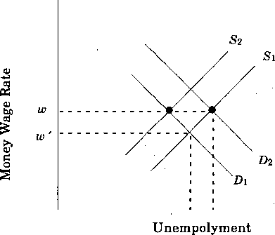
Figure 1. Wage Rates and Unemployment

All four of the responses mentioned above impact on equilibrium wage levels, so it is not too much of an exaggeration to state that regarding unemployment, traditional labor market analysis suggests that “wages alone matter.” This is in marked contrast to the Keynesian perspective that dominated economic thinking from the 1940s through the 1960s that, with little exaggeration, said that “wages do not matter.” A small band of economists, including Ludwig von Mises, F. A. Hayek, Benjamin Anderson and W. H. Hutt, never abandoned the notion that wages are critical in unemployment determination, but these voices carried no weight in the development of the consensus interpretation of why America avoided a depression after World War II.46

Yet the empirical evidence, which suggests that “pent up” demand played no meaningful role for nearly two years in which unemployment stabilized at low levels, is consistent with the theory espoused above. This is not to deny that consumers hungered for consumer goods. Nonetheless, in the critical reconversion period, the growth in actual consumption was modest compared with the reduction in federal defense-related spending.

Table 5
Selected Characteristics of the American Labor Force, June 1945 and June 1946
Labor Force Characteristic	June 1945a	June 1946a
Non-Institutional Populationb	105,290	106,210
Total Labor Force	67,590	62,000
Total Employment	66,700	59,430
Federal Employment	15,849	5,879
Armed Forces	12,130	3,070
Civilian	3,719	2,809
Non-Federal Employment	50,851	53,551
Civilian Employment	54,570	56,360
Male	34,710	39,650
Female	19,860	16,710
Female Civilian Employment as % of Total	36.39%	29.65%
Unemployment	890	2,570
Male	460	2,010
Female	430	560
Unemployment Rate (% of Civilian Labor Force)	1.60%	4.36%
Unemployment Rate (% of Total Labor Force)	1.32%	4.15%
Labor Force Participation Rate	64.19%	58.37%
Employment-Population Ratio	63.35%	55.96%

a Age 14 or over.

b In thousands.

Sources: 1949 Statistical Supplement: Survey of Current Business, p. 53; Monthly Labor Review (August and September 1946).

To begin our look at this evidence, it is interesting to compare labor force statistics at the height of mobilization, June 1945, with statistics just exactly one year later, June 1946 (see table 5).

The total labor pool grew by nearly one million over the year, yet the labor force fell by nearly 5.6 million. The end of the war was accompanied by an enormous drop in the labor force participation rate. In particular, millions of women voluntarily decided to withdraw from the labor force and reverted to their traditional roles as mothers, wives, and housekeepers. About 56 percent of the potential unemployment created by the almost 10 million decline in federal employment was absorbed by voluntary exit from the labor force.

The word “voluntary” in the preceding paragraph is important. It is presumed in a free society that labor voluntarily enters into labor market decisions. Yet during World War II, millions of men were drafted and became part of the labor force; some of them may have not voluntarily been part of that labor force in the absence of conscription. Thus the wartime unemployment rates of under two percent were low, at least in part, because the normal rules of non-coercive labor market participation did not apply. Thus the postwar rise in the reported unemployment rate, modest as it was, still overstated the true recessionary conditions that existed.

Yet the sudden reversion of labor supply to more normal levels was not the only factor in the moderate postwar unemployment. Non-federal employment grew 2.7 million in this first postwar year, in a period before the major consumer goods industries had resumed full production. Indeed, factory employment in June 1946 was still more than 10 percent below the June 1945 levels (because of declining defense-related production), implying the job growth in non-manufacturing, non-federal employment was actually more than four million jobs. More than 27 percent of the problem that the release of 10 million government employees created was eliminated by increased civilian employment, most of it in the private sector. If defense industries are considered, demobilization from June 1945 to June 1946 meant the loss of over 11 million jobs, about four million of which (about 36 percent) were absorbed in the civilian economy.

Why was non-manufacturing civilian employment soaring by over 10 percent in one year, particularly when one considers that economists were widely predicting a resumption of the Great Depression of the 1930s, and when one considers that the mainline durable goods industries (which were in manufacturing in any case) were still at below normal production? How could millions of new civilian jobs be created when there was “underconsumption” by normal standards?

The answer lies, we think, in the other forms of unemployment-determining labor market adjustments discussed above: changes in money wages, prices, and the productivity of labor. The money wage divided by prices is called typically the “real wage.” Real wages adjusted (by division) to take account of productivity changes can thus be called the “adjusted real wage.” It is our contention that, in addition to reduced labor supply, a decline in the adjusted real wage helped absorb the more than 11 million workers released in the first year of the demobilization.

Directly calculating what happened to the adjusted real wages is difficult for a variety of reasons. There is no accepted data series giving hourly wages for the entire labor force before 1947. Annual earnings figures are of questionable value because of a major reduction in overtime work at the conclusion of the war. Regarding prices, the deficiencies of price indices, particularly in a period when price controls are changing, are well known. Similarly, deficiencies in price indices impact on the calculation of labor productivity.

Nonetheless, we calculated the adjusted real wage for labor some 18 different ways, using three different measures of hourly wages, three different price indices, and two different estimates of changing labor productivity. Specifically, we used hourly earnings in manufacturing, retail trade, and contract construction for our money wage measure, and the consumer price index, wholesale price index, and GNP price deflator in calculating real wages, and real private gross domestic product per man-hour, and real private gross domestic product per unit of labor input as our measure of labor productivity.47

The calculations reveal that for 1946, some 14 of 18 estimates show a decline in the adjusted real wage from 1945 levels, with the median decline being 2.35 percent. In no case was there an estimated increase in the adjusted real wage of greater than two percent. Similarly, making calculations for 1947 reveals even more striking results. Some 17 of 18 estimates of the adjusted real wage for 1947 are below 1945 levels (the single exception showed a 0.5 percent increase), with the median estimate recording a decline of 7.15 percent. Using the median, it would appear the adjusted real wage tended to fall some in 1946, and continued to fall in 1947, perhaps explaining the continued robust growth in employment that year.

Elsewhere we have argued that New Deal “underconsumptionist” reasoning led to wage-enhancing legislation that prolonged the Great Depression of the 1930s.48 Some dimensions of reconversion served to reduce (although not eliminate) some deleterious unemployment effects of the New Deal legislative initiatives. For example, the peacetime transition meant a fall in the average work week, as weary wartime workers sought an increase in leisure time. With a fall in the length of the average workweek came a decline, other things equal, in money wages. Suppose a worker making one dollar per hour worked a 45 hour week in early 1945. Because of the Fair Labor Standards Act of 1938, the worker received $1.50 per hour for hours worked past 40, or a total of $47.50 for a 45 hour week, slightly over $1.05 in average hourly pay. A reduction in hours to 40, the nominal hourly wage left unchanged, lowered the paycheck to $40 ($1.00 per hour), a decline in over 5 percent in the average hourly wage. This example was a common occurrence.

Another development, unrealized at the time, was the relative decline in the importance of labor unions in the economy. Labor union membership as a percent of civilian employment reached a peak in 1945 and declined after the war (and has continued to decline ever since). For example, in 1945, union membership equalled 26.59 percent of the civilian labor force; in 1946, the proportion had fallen fairly noticeably, to 25.03 percent, and then to 24.58 percent in 1947.49 The decline occurred despite a rise in the proportion of workers who were male (more inclined to unionize). The decline in relative union importance reduced somewhat the pressures on wage levels that collective bargaining imposes.

At least two factors contributed to the relative decline in union strength. First, the shift in employment from the relatively union-intensive manufacturing sector to the less unionized service sector was a major factor. Even within manufacturing, however, the demise in the War Labor Board after late 1945 removed a pro-union form of governmental intervention. The WLB consistently promoted collective bargaining in war plants and the end of the war brought a close to this activity.

Because of the data problems mentioned earlier in the paper, however, we have only limited faith in the estimates of falling adjusted real wages given above. Fortunately there is an alternative way of discerning the change in adjusted real wages that avoids some of the problems associated with using price indices, etc. When the same price index is used in calculating real wages is utilized in determining what happened to labor productivity, it turns out that the adjusted real wage is simply equal to money wage payments divided by total output or, more appropriately, personal income.

Specifically, real wages are equal to hourly money wages (w) divided by some price index (P), or w/P. Similarly, labor productivity equals money output per hour (O) divided by a price index, or O/P. Assuming the same price index in both calculations, dividing w/P by O/P gives w/O. The latter variable is simply labor compensation as a proportion of GNP or, using distributive shares data, personal income.

Table 6
Compensation as a Percent of GNP and Personal Income, 1945 to 1947
Quarter		Employee Compensation*	Personal Income*	Money GNP*	Compensation as Personal Income	% of: GNP
1945	I	$122.5	$174.4	$222.6	70.2%	55.0%
	II	121.6	174.2	225.0	69.8	54.0
	III	117.4	170.7	213.0	68.8	55.1
	IV	109.1	168.6	200.3	64.7	54.5
1946	I	105.1	168.5	199.1	62.4	52.8
	II	109.8	173.5	206.3	63.3	53.2
	III	114.0	181.4	221.1	62.8	51.6
	IV	116.7	183.8	224.0	63.5	52.1
1947	I	118.5	187.8	228.2	63.1	51.9
	II	119.8	187.6	233.6	63.9	51.3
	III	123.1	196.6	232.4	62.6	53.0
	IV	127.7	201.7	248.6	63.3	51.4

* In billions of dollars.

Sources: 1949 Statistical Supplement, Survey of Current Business (Washington, D.C.: Government Printing Office, 1950), pp. 6, 7; authors’ calculations. GNP statistics differ from those used elsewhere in the paper because of more recent revisions; data for 1945 are not available in those revisions.

Table 6 gives data on employee compensation, personal income and gross national product by quarters. Note that the ratio of employee compensation to income or output falls after the conclusion of the war. Using labor’s share of personal income, the decline is from the 69–70 percent level late in the war to about 63 percent in the 1946 and 1947 quarters. Using labor’s share of GNP, the decline is from 54–55 percent in the late war (first three quarters of 1945) to 51–53 percent in the 1946 and 1947 quarters. However calculated, labor’s share declined, meaning the aggregate adjusted real wage tended to fall. These findings thus are consistent with the results suggested by wage, price, and productivity data. Millions of workers were hired by business despite an uncertain economic future in large part because “the price was right.”

The fall in the adjusted real wage meant an increase in remuneration of capital. After-tax corporate profits, never much over $11 billion on an annualized basis during the war, rose to about $18 billion (on an annual basis) by the last quarter of 1946.50

Nominal interest rates remained extremely low, increasing the spread between anticipated return on invested capital and the cost of borrowed funds. For example, the average interest yield on a triple-A (Moody’s) corporate bond in 1946 was 2.53 percent, the lowest of any year since that statistic has been kept.51 A major factor in the low interest rates, despite a relative tightening in monetary policy, was the government budget surplus that developed in 1946. The federal government, in effect, moved from being a supplier rather than a demander in the loanable funds market. Perhaps the most massive move towards a contractionary (in a Keynesian perspective) fiscal policy in the nation’s history helped to create conditions in capital and money markets that assisted in the transition. The postwar era was a classic case of “reverse crowding out.” Rising profits, and the anticipation of future increases, stimulated investment spending (the only truly robust major component of aggregate demand).

Rising profits led to rising equity values and higher net worths. Raymond Goldsmith estimates the national wealth rose far more in the two years from 1945 to 1947 (46.4 percent) than in the 16 years from 1929 to 1945 (31.1 percent).52 Whereas the anti-capitalistic innovations of the New Deal probably caused what was in real terms a decline in national wealth in the 1929–45 era, the modest but real retreat from interventionism along with a fall in the adjusted real wage and the associated rise in returns to capital led to a significant growth in wealth in the demobilization period.

An excellent case can be made, indeed, that the increase in autonomous consumption in the post-war era reflected increased spending induced by rising wealth. About two-thirds of the shift in autonomous consumption from 1945 to 1947 can be explained by the $267 billion growth in national wealth during that period, if one accepts the Ando and Modigliani view that the marginal propensity to consume out of wealth is about .06.53

In short, rather than “pent-up demand” preventing a depression, the evidence is more consistent with a distinctly non-Keynesian interpretation: A downward adjustment in labor supply and real wages, accompanied by a more responsible (non-deficit) fiscal policy, served to stimulate investment and consumption spending. Relative price adjustments brought about what Keynesians perceived to be an increase in aggregate demand, rather than the other way around.

Conclusions

Modern standard statistical sources suggest there was a very severe economic downturn in 1946. The evidence does not support that conclusion, and it is clear that statistical revisions have served to distort the historical experience. Keynesian economists ex ante predicted a major downturn after the war, but when it did not come they ex post abruptly changed their tune and argued that a surge in private spending, especially consumption and investment spending, prevented a downturn.

The evidence shows that aggregate demand rose too little and too late to explain the low unemployment that prevailed in the first two years after V-J day, the period in which demobilization was completed. What did happen was that labor markets, partially constrained by non-price factors in the wartime period, were allowed to function in a manner that prevented a serious decline. Labor supply abruptly fell, but in addition real wages, adjusted for productivity change, also fell, preventing a massive rise in unemployment.

To the extent aggregate demand was stimulated at all, it was because of the relative price changes outlined above. Lower adjusted real wages meant higher profits and rates of return on investment spending. A dramatic shift in governmental demand for loanable funds, far from contracting the economy as Keynesian economics suggests, kept interest rates at historic lows. Rising wealth associated with the high returns on capital led to increased consumption that ultimately led to a durable goods explosion—but one that took place long after reconversion had occurred without any major unemployment.

Appendix
Estimating the GNP Price Deflator and Real GNP

A model was constructed using real and monetary variables that provided a close statistical fit to the real GNP price deflator for the largely non-price control years 1916 to 1941; the model was estimated by ordinary least squares regression analysis using annual data:

(1) DEFLATOR = 26.895 + 0.326 M2 + 2.717 CPAPER (1.190) (1.573) (3.776)

- 0.000 TONMIL - 0.000 EMPLOY (0.093) (0.012)

R2 = .822, D-W= 1.715, F = 18.521,

where DEFLATOR refers to the GNP price deflator, M2 to that definition of money, CPAPER to the interest rate on commercial paper, TONMIL to the ton-miles of freight hauled by class A railroads, and EMPLOY to the number of employed persons; an autoregressive term is omitted, and numbers in parentheses are t-values.54 The 1942–47 deflator was estimated from (1).

Econometrically Evaluating the “Pent-Up Demand” Argument

A simple bivariate Keynesian consumption function was statistically fitted, where the dependent variable was CONSUMPTION and the independent variable DISINC, for disposable income. Annual data were obtained from Historical Statistics (1975 Edition) for the years 1929 to 1941, and from the same source for 1948 to 1970. In addition, quarterly data for the years 1948 through 1959 were obtained from The National Income & Product Accounts of the United States, 1929–1976. The obtained statistical results follow:

1948–70 : CONSUMPTION = 7.570 + 0.891 DISINC, R2 = .9996,

(4.932) (235.706) D-W = 1.983;

1929–41 : CONSUMPTION = 3.874 + 0.898 DISINC, R2 = .9865,.

(1.882) (29.602) D-W = 1.124;

1948–59 : CONSUMPTION = 9.819 + 0.880 DISINC,R 2 = 9963, Quarterly (4.809) (112.864) D-W = 1.954.

Actual vs. predicted values for 1945–47 using annual data (all dollar numbers in billions) were:

		Predicted Values:
Year	Actual Value	48–70 DATA	29–41 DATA
1945	$119.6	$140.5	$137.9
1946	143.9	149.1	146.6
1947	161.9	158.0	155.5

Using quarterly data for 1948–59, the predicted values for 1946–47 (all dollar numbers in billions) were:

Quarter		Actual Consumption	Predicted Consumption
1946	I	$134.5	$144.5
	II	139.6	147.3
	III	148.4	152.2
	IV	152.7	155.2
1947	I	154.0	155.8
	II	159.0	154.0
	III	163.5	160.3
	IV	167.6	162.4

Postwar consumption did not exceed “normal” levels in relation to disposable income until well into 1947—two years after peak mobilization.

Richard K. Vedder and Lowell Gallaway are distinguished professors of economics and faculty associates of the Contemporary History Institute at Ohio University. Some material is adapted with permission from the forthcoming book Unemployment and the State by Lowell Gallaway and Richard Vedder to be published by the Independent Institute, Oakland, California.

The Review of Austrian Economics, Vol. 5, No. 2 (1991): 3–32

ISSN: 0889–3047

If the weights of the consumption and the government expenditures components of the GNP deflator in this hypothetical example were 60% and 40%, respectively, in 1947, and 80% and 20% in 1948, then the deflator would have risen by 29.4 percent (from 170 to 220) between 1947 and 1948 using 1946 as the base year. If one uses 1949 as the base year, however, we would have calculated an increase of 41.1 percent (from 56 to 79) for the same period.

	1946 as base year		1949 as base year
Year	Consumption Deflator	Government Deflator	Consumption Deflator	Government Deflator
1946	100	100	40	25
1947	105	200	60	50
1948	200	300	80	75
1949	250	400	100	100

1Historical Statistics of the United States, part 1 (Washington, D.C.: 1975), series D-86 for unemployment rates and series F-32 for gross national product. Throughout this article, the standard data series for unemployment rates are used, with recognition that there has been a challenge to the validity of those data during the Great Depression years. See Michael R. Darby, “Three-and-a-Half Million U.S. Employees Have been Mislaid: Or An Explanation of Unemployment, 1934–1941,” Journal of Political Economy 84, 1976.
2A.C. Pigou, Industrial Fluctuations, 1st ed. (London: Macmillan, 1927), p. 176.
3A.C. Pigou, Theory of Unemployment (London: Macmillan, 1933), p. 252. Pigou makes his arguments in a variety of other places. For example, see his “Real and Money Wage Rates in Relation to Unemployment,” Economic Journal 47, 1937, and “Money Wages in Relation to Unemployment,” Economic Journal 48, 1938.
4It is perhaps something of an exaggeration to ascribe this position entirely to Pigou. A number of other economists espoused similar views. Recognizing that the list is incomplete, we cite a few, beginning with Jacob Viner, Balanced Deflation, Inflation, or more Depression (Minneapolis, Minn.: University of Minnesota Press, 1933), especially pp. 12–13. See also W.H. Beveridge, Causes and Cures of Unemployment (London: Longmans, Green and Co., 1931), p. 25, and Unemployment, A Problem of Industry (London: Longmans, Green and Co., 1930), chapter 16; Wilford I. King, The Causes of Economic Fluctuations (New York: Ronald Press Co., 1938), chapter 8; and Lionel Robbins, The Great Depression (New York: Macmillan, 1934).
5John A. Hobson, The Economics of Unemployment (New York: Macmillan, 1923), p. 84.
6W.T. Foster and W. Catchings, Profits (Boston: Houghton Mifflin, 1925) and Business Without a Buyer (Boston: Houghton Mifflin, 1927); and C.H. Douglas, Credit-Power and Democracy (London: C. Palmer, 1920) and Warning Democracy (London: C.M. Grieve, 1931). A more recent interpretation of the Great Depression with underconsumptionist overtones in John Kenneth Galbraith, The Great Crash, 1929 (Boston: Houghton Mifflin, 1976).
7Murray N. Rothbard, America’s Great Depression (Princeton, N.J.: Van Nostrand, 1963), p. 45.
8Henry Ford, The New York Times, November 22, 1929, p. 2.
9The New York Times, November 22, 1929, p. 1. It is interesting to note that Hoover’s inclinations toward underconsumptionism were recognized and, of course, approved, by trade unionists. Witness a statement by the AFL’s John P. Frey in 1929 relating to a public works scheme of Hoover’s. In effect, Frey argued that the president was in agreement with the AFL’s position that depressions were the result of underconsumption and low wages. See Joseph Dorfman, The Economic Mind in American Civilization (New York: Viking Press, 1959), vol. 4, pp. 349–50. See also Ronald Radosh, “The Development of the Corporate Ideology of American Labor Leaders, 1914–1933” (doctoral dissertation in history, University of Wisconsin, 1967).
10Rothbard, America’s Great Depression, chapter 8. Not to be ignored is the fact that ideas such as those that enamored Hoover were not as unorthodox among professional economists as sometimes claimed. See J. Ronnie Davis, The New Economists and the Old Economists (Ames, Iowa: Iowa State University Press, 1971). Davis presents an interesting array of statements by economists and other academics relating to the issue of the impact of wage reductions on the economy (pp. 94–99).
11John M. Keynes, The General Theory of Employment, Interest and Money (London: Macmillan, 1936).
12Abba P. Lerner, “Mr. Keynes’ ‘General Theory of Employment, Interest and Money,’” International Labor Review 34, 1936. See also W.B. Reddaway, “The General Theory of Employment, Interest and Money,” Economic Record 12, 1936. A systematic description of the thought of this time is contained in Lawrence R. Klein, The Keynesian Revolution (New York: Macmillan, 1947). For a taxonomic description of the various views of the aggregate demand schedule for labor, see Sidney Weintraub, “A Macroeconomic Approach to the Theory of Wages,” American Economic Review 46, 1956.
13Paul M. Sweezy, personal letter to John B. Shelley, dated February 11, 1977, cited in Dana C. Hewins and John B. Shelley, “Sweezy’s Kink: Macro Foundations of a Micro Theory,” Economic Inquiry 17, 1979.
14For a description of the various dimensions of the Keynesian critique of classical economics, see Alvin H. Hansen, A Guide to Keynes (New York: McGraw-Hill, 1953). More recent appraisals and restatements of the total thrust of Keynesianism are Abba P. Lerner, “From ‘The Treatise on Money’ to ‘The General Theory,’” Journal of Economic Literature 12, 1974; and Hyman P. Minsky, John Maynard Keynes (New York: Columbia University Press, 1975).
15Peter Temin, Did Monetary Forces Cause the Great Depression? (New York: Norton, 1976), p. 140. Temin also attempts to demonstrate that the Great Depression was brought on by an autonomous shift in the consumption function. That view has been challenged (successfully, we think) by Thomas Mayer, “Consumption in the Great Depression,” Journal of Political Economy 86, 1978.
16Keynes, The General Theory. In chapter 2, Keynes is very explicit. In reference to the principle that real wages and employment are systematically related, he says, “I am not disputing this vital fact which the classical economists have (rightly) asserted as indefeasible.”
17Ludwig von Mises, The Theory of Money and Credit (New Haven, Conn.: Yale University Press, 1953). Permission granted by Mrs. Margit von Mises. Quotes from 1981 Liberty Classics, Indianapolis, edition.
18Milton Friedman, “The Role of Monetary Policy,” American Economic Review 58, 1968.
19In particular, see Jerome Stein, Monetarist, Keynesian, and New Classical Economics (Cambridge, United Kingdom: B. Blackwell, 1982).
20The key assumptions are constant returns to scale and neutral disembodied technical progress.
21The underlying statistical models are moderately complex. They are described briefly in the statistical appendix. The logic and structure of the models are more fully developed in Lowell Gallaway and Richard Vedder, The “Natural” Rate of Unemployment, staff study, Subcommittee on Monetary and Fiscal Policy, Joint Economic Committee, Congress of the United States (Washington, D.C.: 1982).
22Federal Reserve Bulletin, various issues.
23Historical Statistics, series D-86.
24The productivity-adjusted real wage rate on a quarterly basis is calculated by dividing the manufacturing wage bill by the product of Federal Reserve Board (not the wage bill) and the index of average labor productivity (not total output) should be used. However, converting the wage bill and the index of industrial production to wage rate and productivity measures involves dividing both of them by the same quantity of labor (L). Since L appears in both the numerator and denominator of the expression for the adjusted real wage rate, it cancels out and can be ignored.
25As calculated from Historical Statistics, series D-688.
26Ibid,, series D-683 and D-688.
27Ibid., series D-724 and Paul A. David and Peter Solar, “A Bicentenary Contribution to the History of the Cost of Living in America” in Paul Uselding, ed., Research in Economic History, vol. 2 (Greenwich, Conn.: JAI Press, 1977), pp. 59–60.
28Broadus Mitchell, Depression Decade, vol. 9, The Economic History of the United States (New York: Rinehart, 1947), p. 84; and Arthur Schlesinger, Jr., The Age of Roosevelt: The Crisis of the Old Order, 1919–1933 (Boston: Houghton Mifflin, 1957), p. 249. Interestingly, though, some observers of the period disagree with this assessment. For example, Leo Wolman, Wages in Relation to Economic Recovery (Chicago: 1931) notes, “[I]t is indeed impossible to recall any past depression of similar intensity and duration in which the wages of prosperity were maintained as long as they have been during the depression of 1930–1931.” Similarly, Don Lescohier, “Working Conditions,” vol. 3, History of Labor in the United States, 1896–1932, John R. Commons and Associates, eds. (New York: Macmillan, 1935) states:
29Historic Statistics, series D-802, D-813, D-818, and D-824, respectively.
30Robbins, The Great Depression, p. 224.
31Geoffrey H. Moore, ed., Business Cycle Indicators, vol. 2, Basic Data on Cyclical Indicators (Princeton: Princeton University Press, 1961), p. 129.
32Benjamin M. Anderson, Economics and the Public Welfare (New York: Van Nostrand, 1949), p. 72.
33Historical Statistics, series D-839.
34Anderson, Economics, p. 220.
35Without the productivity adjustment, real wages in manufacturing (in 1923 prices) rose from 58.9 cents an hour in December 1929 to 62.5 cents an hour in December 1930. After that, they continued to rise to 66.3 cents an hour in January 1932. Wilford I. King, Causes of Fluctuations, pp. 182–83. See also Sol Shaviro, “Wages and Payroll in the Depression, 1929–1933” (unpublished M.A. essay, Columbia University, 1947).
36Milton Friedman and Anna J. Schwartz, A Monetary History of the United States, 1867–1960 (Princeton, N.J.: Princeton University Press, 1963).
37U.S. Bureau of the Census, National Income and Product Accounts of the United States, 1929–1976 (Washington, D.C., Department of Commerce, Bureau of Economic Analysis, 1981), p. 308.
38Moore, Business Cycle Indicators, p. 106.
39Harold Barger, Outlay and Income in the United States, 1921–1938 (New York: National Bureau of Economic Research, 1942), appendix B, table 28. A smaller profit decline is reported in a less comprehensive survey conducted by the Federal Reserve Bank of New York. See Irving Fisher, Booms and Depressions: Some First Principles (New York: Adelphi, 1932), p. 98.
40Robbins, The Great Depression, p. 205. The data were originally published in Commercial and Financial Chronicle.
41This is based on the Standard and Poor’s index, which fell 32.9 percent from September to November 1929. The second decline actually began in April 1930. A similar pattern is observed using the Dow-Jones index, which fell 39.7 percent from April to December 1930, compared to 37.0 percent from September to November 1929. The recovery in stock prices after November 1929 was robust; the April 1930 Dow-Jones index was the eleventh highest recorded in history, exceeded only in the first ten months of 1929. See Moore, Cyclical Indicators, pp. 108–9.
42Ben Bernanke, “Nonmonetary Effects of the Financial Crisis in the Propagation of the Great Depression,” American Economic Review, June 1983, p. 261.
43Ibid., p. 262.
44Federal debt declined about $700 million in both 1929 and 1930, but rose more than $600 million in 1931. See Historical Statistics, series Y-493.
45If one uses the consumer price index to measure price changes, real interest rates on bank loans in 1929 averaged about 6 percent, rising to about 7.7 percent in 1930, and to about 13 percent in 1931. This is based solely on current year price changes. A real interest rate model using weighted averages of past price changes would show a smaller rise. Interest rate data are based on Federal Reserve System reports. See Moore, Cyclical Indicators, p. 154.
46Historical Statistics, series F-54.
47Friedman and Schwartz, A Monetary History, table A-1, pp. 712–13.
48Ibid., table B-3, p. 803.
49Ibid. The deposit/currency ratio fell from 11.57 in October 1929, to 4.44 in March 1933, a decline of 7.13 points, with 3.87 points (54 percent) of that decline occurring between October 1930 and October 1931.
50Ibid., pp. 308–13.
51The price would fall to $750 only for a consol, a bond with no maturity. Short-term bonds would sell at a small discount from face value because the owner of the bond would receive the face value at maturity.
52Historic Statistics, series X-581.
53Capital accounts were $10,372 million. Ibid., series X-587.
54Most nominal interest rate series show little change in the early years of the Great Depression, and, indeed, many show some decline. This masks two phenomena, however. First, declining commodity prices during the period led to rising real interest rates over time. Second, most interest rate series report actual transactions, probably ignoring a growing number of customers who were crowded out because of sharply rising risk premiums. It is possible that interest rates demanded of some average potential borrower rose, even though actual interest rates reflected in transactions did not rise.