Review of Austrian Economics

The Recession of 1990: An Austrian Explanation

Arthur Middleton Hughes

In the misdirection of labor and the distortion of the structure of production during past business cycles, it was fairly easy to point to the places where the excessive expansion had occurred because it was, on the whole, confined to the capital goods industries . . .

In contrast, the present expansion of money, which has been brought about partly by means of bank credit expansion and partly through budget deficits, has been the result of a deliberate policy and has gone through somewhat different channels . . .

I do not doubt that in a sense we have today the same kind of phenomenon, but the over-expansion, the undue increase of labor employed in particular occupations, is not confined to a single, clearly defined block such as the capital-goods industries. It is now spread much more widely, and the distribution is much more difficult to describe. It is a field I would wish some statistically minded economist would investigate in order to show how the process operated in particular countries.

Friedrich A. Hayek1

Why do we have booms and recessions? The conventional Keynesian view is that recessions are a failure of consumer demand. Keynesians, however, are not entirely clear on why consumers periodically act in unison to reduce their consumption. A more logical answer to the question is the Mises—Hayek theory of the business cycle. The ideas of Ludwig von Mises and Friedrich A. Hayek, central to the Austrian school of economics, suggest an entirely different approach to the business cycle from what has become the conventional wisdom for the last 40 years. It is the purpose of this paper to explore the Austrian explanation of the business cycle, sometimes called the Austrian business cycle theory (ABCT), and to apply that theory to the recession of 1990–1992.

The Structure of Production

The Austrian view of the economy differs substantially from that of Keynesians or monetarists in their treatment of capital. Keynesians tend to lump the capital accumulated by various industries throughout the country into an amorphous and given “stock of capital.”2 Investment by business is treated in GNP analysis as a single variable, regardless of the type of business in which the investment takes place. Both Keynesians and Monetarists tend to deal with aggregates in explaining business cycle theory whereas, as pointed out by James Clark and James Keeler, “macroeconomic aggregates are not considered meaningful concepts by the Austrians who are more concerned with relative changes among the components of the aggregates.”3 In fact, the whole concept of the Gross National Product, as defined in conventional economics today, leaves out of the analysis more than 40 percent of the industrial activity going on every year—the activities in the higher stages of production.4

Austrian economists see the industry of any developed economy as a progression of activities from the most basic extraction of materials from the earth (by means of mining, forestry, fishing, or farming), through the production of semi-finished goods (such as lumber, steel, chemicals, and machinery), down to the production and sale of final goods and services to consumers.5

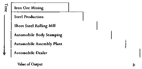
Figure 1. The Structure of Production

One big difference between the companies in different levels in the structure of production is the time that must elapse before their investments return a profit: see figure 1. A retailer may add a distribution warehouse, and begin to make a profit from it right away, in terms of having more stock on hand, fewer back orders, or greater ability to satisfy the consumer.

A higher-stage firm, such as a coal mine or primary metal producer, often has a much longer lead time. It may take five or ten years before a new plant can be built, equipped with proper machinery, staffed with trained workers, and put into full operation such that the profits from operations will begin to amortize the original investment.

Austrian economists add to this another reason for the different impact of interest rates on different levels of the structure of production. In the absence of governmental interference, interest rates in the market are determined by the interactions of the differing time preferences of borrowers and lenders of money. Interest rates send valuable and important signals to market participants. These signals have different meanings to industries depending on where they are on the structure of production. Higher-stage industries are far removed in time from the ultimate consumers. They must, as a result, use prices and interest rates as important messages about the state of the market. Lower-stage industries do not need these messages as much, since they meet daily with the consumers and can judge demand directly. It usually takes a long time for goods and services produced in higher stages to reach the ultimate consumer. A bar of iron, for example, may go through dozens of stages before it emerges as a rotor on a fan in someone’s personal computer. Someone has to pay the interest charges on that piece of iron while it waits, in factory after factory, to be transformed, finally, into something that a consumer would want to buy. Higher-stage producers, therefore, without realizing it, must carry the burden of subsequent interest charges which, if the interest rates increase too much, will affect the sales of the consumer products made out of their output. Lower-stage producers, who are closer to the consumer in time, do not have to carry the same interest burden, and so are less affected by changes in rates.

Because of these dissimilarities, changes in the cost of capital result in very different investment patterns. For a lower-stage industry (such as a retailer, wholesaler, or food producer), the cost of capital is not as important, because the interest charges do not have to be carried very long before the payout begins. For a higher-stage industry, increases in the cost of capital often mean the difference between undertaking a new project or not doing it at all.

Why Industries Differ in Capital Needs

To illustrate the difference, consider two different industries: a food retailer and a primary metals manufacturer.

The food retailer is selling a perishable commodity. He has few warehouses. Most of his capital is tied up in goods on display in his stores. Movement of stock is brisk. If he were to add a new store, a warehouse, or additional trucks, he would expect to build or buy them rapidly, and have them earning income within a year or so of the purchase decision. If the interest rate is 8 percent, or 12 percent—it does not matter very much. At 12 percent, he may hesitate to build a new store but he will still add to his truck fleet.

The primary-metal manufacturer has a very different attitude. Modern metal extraction and production involves environmental questions, very elaborate and expensive capital equipment, and many years of planning. A new steel, copper, or aluminum plant may cost many hundreds of millions of dollars, and take 10 years from site purchase to full production. Here, the interest rate is everything.

Suppose that the cost of a new plant is $200 million, and that it will pay a return of $40 million per year when it is completed. At a market rate of interest of 12 percent, such a plant would be worth $333 million. Time is money. How long would it be before the cost of interest payments would drive the original investment of $200 million up over $333 million? In other words, how much time does the firm have to build the plant before the investment is no longer profitable? The formula for the long term value (V) of an investment which yields Y amount per year when the market rate of interest is (r) is:

= Y/r

V = $40/.12

V = $333

The formula for the cost (C) including interest of an investment (I) for n years at (r) rate is:

C = 1(1 +r)n

Solving for n, the formula becomes:

n = Log(C/I) / Log(1 + r)

The maximum time that an investor can afford to wait for his return is thus based both on the rate of interest, and the value of the expected yield in relation to his investment. His maximum time is when C = V If we substitute the value of the investment (Y/r) for C in the above formula, it becomes:

n = Log(Y/(I * r))/Log(1 + r)

If the interest rate is 12 percent, the plant must be up and running in four-and-a-half years, or the cost will exceed its market value.

n = Log(40/(200 * 0.12)) / Log(1.12)

n = 4.5 years.

On the other hand, if the market rate of interest is 8 percent, the value of the same plant that returns $40 million per year is $500 million. At 8 percent per year, how long will it be before interest payments have forced an original investment of $200 million up to $500 million?

n = Log(Y/(I * r)) / Log(1 + r)

n = (log(40/(200 * 0.08))/ Log(1.08)

n = 11.9 years

So, at 8 percent they can afford to take a maximum of 11.9 years to build the plant before it is no longer profitable. Most higher-stage investments take longer than four-and-a-half years before they begin to pay dividends. Most lower-stage investments take much less time than that.

What this tells us is that the market rate of interest means different things to different segments of the structure of production. When rates go down, a great many higher stage projects that were uneconomic at high interest rates become at once feasible. When rates go up, many higher-stage long-term projects have to be scrapped. These simple rules do not apply to lower-stages of production, simply because their payoff times are much shorter. They don’t have to pay as much interest on their typical project. A lower stage producer is less likely to embark on an investment project.

Why the Money Supply is Expanded

Western governments since the 1940s, following Keynesian principles, have increased their money supplies every year, thus leading to constantly-rising prices believing that it was good for their economies. They have also found that inflation is a good way to finance their governmental-spending programs without the need to increase taxes—the increased spending also being a Keynesian prescription for achieving full employment. How much increase in the money supply is the desirable goal? Keynesians and many monetarists would favor an annual increase of 5 to 6 percent per year.6

A laissez faire system is doomed to wasteful ups and downs of the business cycle and perhaps to long fits of stagnation. . . . Simple capitalism has been replaced virtually everywhere by the mixed economy (a “welfare and managed economy”). Everywhere in the Western world, governments and central banks have shown they can win the battle of the lasting slump if people want them to . . . Just as we no longer meekly accept disease, we no longer need accept mass unemployment.7

The core of the Austrian macroeconomic theory is that government “fine tuning of the economy,” through government-orchestrated expansions and contractions of the money supply, are actually the cause of business cycles because of the differing impact of the resulting interest rate changes on different stages in the structure of production. Roger Garrison has pointed out that Mises and subsequent Austrian theorists, influenced by Knut Wicksell, see a “distinction between the natural rate of interest and the bank rate of interest” and recognize “that the bank rate can diverge from the natural rate. . . The institutional setting in which the interest rate reflects both the intertemporal preferences of market participants and the actions of policy makers, then, figures importantly in the Austrian account of the artificial boom and inevitable bust. Fritz Machlup accurately summarized the Austrian view with the statement that ‘monetary factors cause the cycle but real phenomena constitute it’. . . . The focus of the Austrian theory is on the actual market process that translates the monetary cause into the real phenomena and hence on the institutional setting in which this process plays itself out.”8 Here is the way it works.

The Austrian Explanation of the Business Cycle

When the money supply is expanded, the cost of capital comes down. Industries in higher stages find that many of their long-term projects are now feasible. They begin to build new productive facilities which have long-term payouts. To build these plants, they have to hire more workers which they pay with borrowed money. The hiring of workers, and the competition for capital equipment and resources, bids up the prices of goods and the wages of the workers, and increases interest rates. The rising rates put more pressure on the government to ease up credit by further increases in the money supply.

The increased money supply affects mainly the higher stages of production, not the lower stages, because it is higher stages that depend on long-term external capital infusion to undertake their development projects. Eventually, of course, the expansion also affects the lower stages, as highly-paid workers spend their wages on more consumer goods. A boom is in the making.

As long as the government keeps feeding the boom with more and more money, the good times roll. Higher-stage industries undertake more and more costly projects, and more and more workers move to those sectors. Their spending fuels the activities in other sectors, and their absence raises the wages of those still remaining in these sectors. Now all levels of production are competing for loanable funds. The game is up when the monetary authorities finally become alarmed at the level of price increases, and muster the courage to reverse their expansionary course, usually by raising the discount rate or selling bonds on the open market.9 At this point, the good times come to an end. The expanded spending by consumers tends to force the interest rates back up.

The Coming of the Recession

The inflating economy is like a giant pyramid scheme. As long as the government keeps pouring money in, the system will keep going. Once the government stops, a recession is inevitable.

The first to go will be the long-term capital projects. As interest rates go up, new projects not yet started will be canceled. But many of those which are only half finished will also have to be abandoned. One reason is that capital financing is often obtained on a pay-as-you-go basis. As industries compute the payoff for a project started when interest rates were 8 percent, which now must compete for funds at 12 percent, they realize that the project is a loser. They cut their losses, and abandon the enterprise. The workers are laid off, and often, much of the project is a total loss. The reason? Because most capital goods (semifinished goods and facilities) are specific to an industry, and have little general usefulness. It becomes apparent that much of the expansion undertaken in prior years was really false expansion, based not on a truly-growing economy, but on the government inflation of the money supply. As workers are laid off in higher-stage industries, they reduce their spending for consumer goods. The recession spreads.

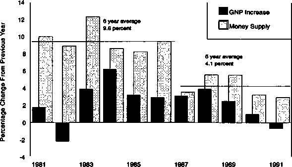
Figure 2. Money Supply Increase versus GNP Increase 1981–1991

Source: Economic Report of the President 1992 M = M2

The Recession of 1990

The process just described took place during the years from 1981 to 1992. From 1981 to 1986 (and earlier), the Federal Reserve embarked on a massive increase in the money supply which averaged 9.6 percent per year while the GNP in real terms expanded by only 2.6 percent. From 1987 to 1991, the money supply increased by an average of only 4.1 percent per year while, the GNP increased by about 2 percent.10 The dramatic drop in government money supply expansion is shown by Figure 2.

The money supply expansion from 1981 to 1986 resulted in expanded bank loans to higher-stage industries, while lower stage industries, at first, were unaffected. As more workers were hired by these expanding industries, and others received pay increases and began to spend their pay on increased consumer goods, the lower-stage-industry bank borrowing increased. Lower-stage capital expansion is based more on anticipated consumer demand than upon the availability of capital. The precipitous drop in government money supply expansion after 1986 ended the boom in the higher-stage industries. This was the beginning of the recession—although it did not show up for four more years.

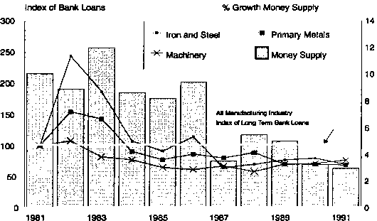
Figure 3. Long-Term Bank Loans by Higher-Stage Industries 1981–1991 All Manufacturing Bank Loans = 100

Source: Quarterly Financial Report, Census Bureau and Federal Reserve

Figure 3 depicts long-term bank loans to higher-stage industries (represented by iron and steel, primary metals, and machinery) relative to total-long-term bank loans to all manufacturing industries, superimposed on the annual growth of the M2 money supply. Notice how two of these industries increased their loans, in relation to all manufacturing loans, dramatically during 1982 and 1983. The increase was 250 percent in iron and steel and 150 percent for primary metals. Machinery industries—much lower in the structure of production than primary metals—increased their borrowing only slightly during the expansionary period and were generally below industry averages thereafter.11

The fact that the increases in higher stage borrowing from 1981 to 1985 were based on the increased availability of capital funding rather than directly anticipated demand for increased output is shown by the statistics on industrial production during this period. The level of production in the iron and steel industry at the time was far below capacity (estimated at about 63.5 percent from 1981 to 1985)12 due to the low level of orders. Lower-stage industries, closer to the consumer, showed no such increased borrowing levels during this period of massive money supply increases.

With the benefit of hindsight, we know today that net shipments of steel mill products would never regain their 1981 levels during the following decade. Why did they expand their production? All that industry participants knew at the time was that funding for expansion was available. Iron-ore production, much closer to its direct customers than the iron and steel industry, did not invest in expansion during the period, and, in fact, closed down several of its operating mines.13

When the massive money-supply increases came to an end in 1986, the iron and steel industry collapsed. Prices of their product dropped every year as the higher-capacity and more-efficient new facilities competed with the older plants for what was essentially a disappointing demand.

For the copper industry 1981–1985 were turbulent years. They were years of bankruptcies, shut down mines, laid off workers. But financing was available. Despite massive losses in the industry, Standard Oil of Ohio invested $400 million to modernize Kennecott’s Utah Copper Division early in the period. After serious losses, the plant was shut down entirely in 1985.14

In looking at these figures, it is important to recognize that these numbers are industry averages only. Inside each number are dozens, or hundreds or thousands, of individual firms—some of which were borrowing heavily, others of which may have been doing nothing in the way of external financing. When the figures for an entire industry are shown to be at 270 percent of their previous level, this must mean that some individual firms had really increased their bank borrowing by a major amount. For primary metals, for example, bank loans in the first quarter of 1981 were listed at $4,010 million. By the first quarter of 1982, their level was $7,597 million. Iron and steel had a similar increase: from $1,832 million to $5,453 million. Machinery bank loans increased from $7,898 in 1981 to $10,428 millions by 1982.

But for iron and steel, and primary metals, the borrowing surge stopped after 1984. Thereafter, their bank borrowing was less, proportionately, than the level of all manufacturing. The impact that money-supply increases produce on higher-stage investments is well illustrated by the activities of these two industries.

Lower-Stage Industry Long-Term Borrowing

Contrast this higher-stage borrowing and capital spending with the bank borrowing of lower-stage industries during the same period (1981–1991). Food, rubber, and textiles are industries that are much closer to consumers than are iron and steel and primary metals. We could have also looked at petroleum, drugs and motor vehicles as representative of lower-stage industries, but for special demand reasons, one could argue that the 1980s were not typical years for these groups.

Drugs were affected by the growth of the Medicare and Medicaid programs which began to be important during this period. American motor vehicles were competing heavily, for the first time, with the Japanese. Petroleum is a vertically-integrated multi-national industry with high capital investments in higher-order (drilling) and lower-order (refineries and gas stations) goods.15

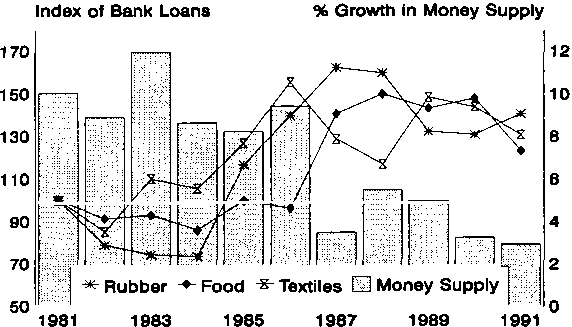
Figure 4. Long-Term Bank Loans by Lower-Order Industries, 1981–1991 All Manufacturing Bank Loans = 100

Source: Quarterly Financial Reports 1962–1992, Census Bureau, and Federal Reserve.

Figure 4 depicts the long-term bank borrowing of three lower-stage industries during 1981–1991 as contrasted with total long-term bank lending to manufacturing industries during the period and the growth in the money supply. Our three lower-stage industries illustrate the Mises—Hayek theory. During the period of money supply expansion from 1981 to 1984, they generally maintained their bank loans virtually unaffected by the expansion of loanable funds. Towards the end of the expansion period, textile and rubber industries began to undertake long-term projects that pushed them up to 170 percent and 200 percent of industry averages by 1986. By 1987 consumer spending had driven even food industries to compete for bank-loan funds at a very high rate.

Notice that the peak borrowing for food and rubber came after 1986—at a time when the money-supply growth rate was being drastically curtailed. Why was that? The previous expansion in higher-stage industries produced an increase in consumer spending which pushed lower-stage manufacturers to borrow to expand their facilities to meet it.16

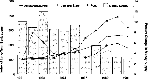
Figure 5. Long-Term Bank Loans to Industry 1981–1991

Source: Quarterly Financial Report 1982–1992 and Federal Reserve 1981 = 100.

Figure S puts the entire period into perspective. It shows total dollar borrowing by all manufacturing industries adjusted for inflation—the producer’s price index. As you can see, long-term bank borrowing by manufacturing industries increased steadily from 1981 to 1991.17 The dramatic reduction in money supply increases in 1987 did not affect the total borrowing level at all—in fact the average annual increase in borrowing after 1986 was higher than before 1986. What did change was the distribution of that borrowing. Before 1986, most of the increase was led by higher-stage industrial borrowers, represented here by iron and steel. After 1986, the increase in total borrowing was fueled by lower-stage industries, represented here by food.

Most traditional economists looked on the years from 1986 through 1988 as being boom years. They overlooked what was happening in higher-stage industries. What was going on in iron and steel, for example was this: LTV Corp., Wheeling-Pittsburgh Steel Corp. and Sharon Steel Corp., were all forced to file for bankruptcy following the collapse of steel demand in 1985 and 1986. This collapse accelerated the reduction of U.S. steel-making capacity, and triggered a major restructuring of the iron ore and steel industries on both sides of the U.S.-Canadian border.18

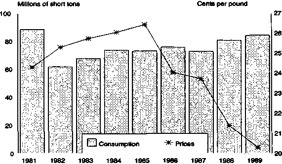
Figure 6. Iron and Steel Consumption and Prices

Source: Minerals Yearbook 1989

Figure 6 shows what happened to steel prices after the Federal Reserve stopped inflating the money supply. Consumption of steel failed to regain its 1981 levels in the subsequent decade.

The situation in copper was quite different, but illustrative of the same basic problems. Coinciding with the United States money-supply increases which began in 1981, the U.S. copper industry began a major inventory increase to 275 percent of 1979 levels by 1983. Beginning in 1984, inventories began to fall drastically every year until 1988, until they reached an average of about 14 percent of 1981 levels by 1989.19

In figure 7, we contrast long-term borrowing of all manufacturing, retailing, and wholesale firms. Retail borrowing took a nosedive from 1981 to 1982—recession years—and stayed down all during the period when the Federal Reserve was inflating the money supply. Retail borrowing only accelerated in 1987—after the inflation of the money supply was over! Why? Because retail firms borrow to meet immediate customer demand. Higher-order firms borrow when financing is available on attractive terms.

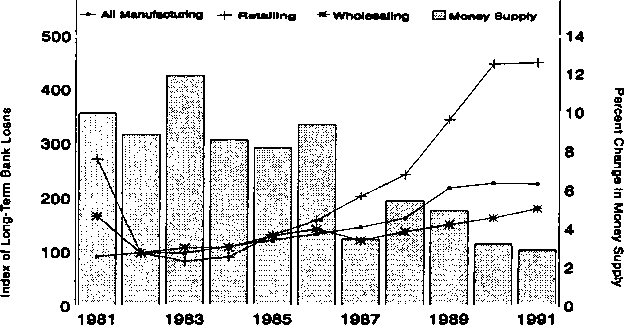
Figure 7. Bank Loans to Manufacturing, Retailing, and Wholesaling

Source: Quarterly Financial Report 1982–1992 and Federal Reserve 1982 = 100, adjusted for Producers Price Index

In the later stages of the boom, consumer spending competes with and overtakes all other types of activity. It is at this point that unused higher-stage capacity materializes because, as Hayek says, “We are unable to use the fixed plant to the full extent because the current demand for consumer’s goods is too urgent to permit us to invest in current productive services in the long processes for which (in consequence of ‘misdirections of capital’) the necessary durable equipment is available.”20 In the last part of the decade, retail use of loan funds, secured to meet expanding consumer spending, dwarfed the growth rates of manufacturing and wholesaling borrowing activities. In a contest, lower stages always win.

The data assembled here provide an illustration of the working of Austrian business cycle theory,21 namely, that business cycles are caused by government inflation of the money supply, leading to excessive borrowing by higher-stage industries. This borrowing produces a boom which must come to an end when the inflationary activities stop—as they must, when the government can no longer continue to stoke the monetary fires with more and more monetary expansion. The end of the boom leads to a crack-up and a recession.

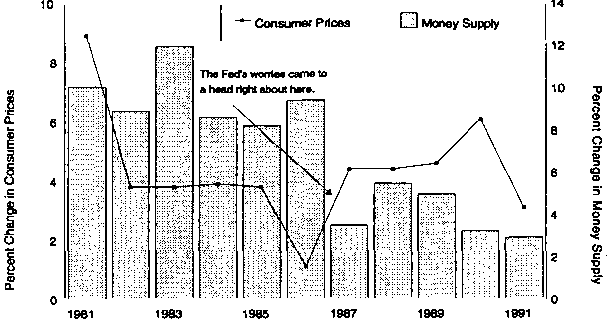
Figure 8. The Fed Loses Its Nerve

Source: Bureau of Labor Statistics and Federal Reserve

The recession did not begin until 1990, but the seeds were planted in 1981–1986, with the money supply expansion. The recession was triggered in 1987 when the Federal Reserve lost its nerve to continue the inflationary spiral. What caused the Federal Reserve to alter its policy so drastically in 1987?

1987: The Fed Lost Its Nerve

Why the Federal Reserve alters its policies is always a matter for speculation. It is seldom one single thing that is crucial. The Fed worries about inflation, deficits, the money supply, interest rates, and unemployment. But certainly a key concern in the past 20 years has been the value of money, as represented by the consumer price index.

Figure 8 shows one key variable—the consumer price index—against the annual growth rate of M2. The Fed pursued a high inflation policy for 6 years. During all of these years, prices were flat or falling. Then, in 1986, prices began to climb. Eight years previously, in the fall of 1979, the Federal Reserve changed its policies dramatically when it decided to clamp down on double-digit inflation. Its actions produced the recession of 1982, and a halt in the inflationary spiral. Price increases from 1982 through 1985 were held to a flat 3.8 percent per year. The shift was welcome news for the public and for businessmen generally. When price increases in 1986 dropped to a low of only 1.1 percent, there was rejoicing in all quarters. But while the Fed leaders were happy about the price levels, there was real concern about the growth of the money supply. Even the non-Austrian Fed economists realized that the country would have to pay for the excessive growth in money at some point. The year 1987 looked like that point.

Consumer price increases, led by medical costs due to Medicare and Medicaid, began to zoom up. When the 1987 rise passed the 3.8 ceiling and kept on rising, the Fed lost its nerve. It put the brakes on money supply increases in a drastic way, and kept them on for the next 5 years. Some would point to this decision and say that the recession of 1990–92 was caused by Fed actions in 1987. That may be true. But Austrians know that that is not the whole story. The actions which led to the recession really took place from 1981–86. Once the money supply was inflated during this period, the actions of 1987–1991 were inevitable, and so was the recession.

During the time between 1987 and 1990, the public was unaware of the time bomb ticking away. Life went on as usual. New businesses were formed at an expanding rate, and business failures were on the decline. Corporate profits from 1987 to 1989 rose by 31 percent. Consumer prices rose by 4.4 to 6.1 percent. Mortgage debt rose by 48 percent from 1986 to 1990, and consumer credit rose by 22 percent in the same period.22 None of the standard signals showed to Keynesian economists any sign of the impending recession, for one very simple reason: they were looking in the wrong place.

Conclusion

Deficit spending and money-supply expansion do not eliminate recessions. They cause recessions. This fact will never be understood unless economists and government policymakers stop trying to micro-manage the economy, and start studying what their actions are doing to the structure of production. Heavy inflation of the money supply followed by sharp cutbacks change the rules right in the middle of the game for millions of businesses in the economy.

For the last 40 years, government expansionary policies have stimulated industries to create false and untenable investments. These policies are followed by government corrective actions that destroy those same projects—waste the billions of dollars invested in them, and throw millions out of work. Business cycles are not an essential feature of market capitalism. They are the result of government interference with the market.

Arthur Middleton Hughes is an adjunct professor of economics at the University of Maryland.

Review of Austrian Economics 10, no. 1 (1997): 107–123

ISSN: 0889–3047

	Millions of Dollars	Percent
Gross Intermediate Products	$3,297,977	43.8
Gross National Product	$4,235,116	56.2
Gross National Output	$7,533,093	100.0

	Long-Term Loans		Long-Term Loans
All Manufacturing	74,129
All Durable	39,198	All Non-Durable	34,931
Stone, Clay	2,431	Food	7,364
Primary Metals	7,597	Textile Mill	1,824
Iron Steel	5,453	Paper	2,222
Non Ferrous	2,144	Printing & Publ	3,656
Fabricated Metals	4,575	Chemicals	5,238
Machinery	10,428	Indus Chem	2,346
Electrical	3,870	Drugs	352
Transport	4,627	Petroleum & Coal	6,919
Motor Vehicles	1,211	Rubber	1,737
Aircraft	1,802	Other Non-Durable	2,158
Instruments	1,296
Other Durable	4,373

Note: The figures do not add up to the total because they are a selection from a large government survey. The selection of industries to illustrate this paper was a subjective one. The statistics in the survey were not collected based on the stage of production. Every industry grouping for which statistics exist is a combination of different heterogeneous companies making different products. I picked the groupings (iron and steel, primary metals, food, textiles, rubber, wholesaling, and retailing) because they seemed to, in general, represent examples of higher-order and lower-order industries. They help to illustrate the Mises-Hayek trade-cycle theory. These examples do not prove the validity of the theory, which is an apriori statement which does not require empirical verification.

The best government source which provides a breakdown relevant to the structure of production is a survey done every 5 years by the Department of Commerce, called the “Interindustry Structure of the United States,” based on work by Wassily E. Leontief, whose first tables were prepared for 1919, 1929, and 1939. It provides a rough guide to understanding the position of the industries in the QFR, although not a definitive one.

Thousands of Metric Tons
1980	91,983
1981	97,903
1982	57,203
1983	63,050
1984	68,450
1985	66,049
1986	57,513

• 1Historical Statistics of the United States, part 1 (Washington, D.C.: 1975), series D-86 for unemployment rates and series F-32 for gross national product. Throughout this article, the standard data series for unemployment rates are used, with recognition that there has been a challenge to the validity of those data during the Great Depression years. See Michael R. Darby, “Three-and-a-Half Million U.S. Employees Have been Mislaid: Or An Explanation of Unemployment, 1934–1941,” Journal of Political Economy 84, 1976.
• 2A.C. Pigou, Industrial Fluctuations, 1st ed. (London: Macmillan, 1927), p. 176.
• 3A.C. Pigou, Theory of Unemployment (London: Macmillan, 1933), p. 252. Pigou makes his arguments in a variety of other places. For example, see his “Real and Money Wage Rates in Relation to Unemployment,” Economic Journal 47, 1937, and “Money Wages in Relation to Unemployment,” Economic Journal 48, 1938.
• 4It is perhaps something of an exaggeration to ascribe this position entirely to Pigou. A number of other economists espoused similar views. Recognizing that the list is incomplete, we cite a few, beginning with Jacob Viner, Balanced Deflation, Inflation, or more Depression (Minneapolis, Minn.: University of Minnesota Press, 1933), especially pp. 12–13. See also W.H. Beveridge, Causes and Cures of Unemployment (London: Longmans, Green and Co., 1931), p. 25, and Unemployment, A Problem of Industry (London: Longmans, Green and Co., 1930), chapter 16; Wilford I. King, The Causes of Economic Fluctuations (New York: Ronald Press Co., 1938), chapter 8; and Lionel Robbins, The Great Depression (New York: Macmillan, 1934).
• 5John A. Hobson, The Economics of Unemployment (New York: Macmillan, 1923), p. 84.
• 6W.T. Foster and W. Catchings, Profits (Boston: Houghton Mifflin, 1925) and Business Without a Buyer (Boston: Houghton Mifflin, 1927); and C.H. Douglas, Credit-Power and Democracy (London: C. Palmer, 1920) and Warning Democracy (London: C.M. Grieve, 1931). A more recent interpretation of the Great Depression with underconsumptionist overtones in John Kenneth Galbraith, The Great Crash, 1929 (Boston: Houghton Mifflin, 1976).
• 7Murray N. Rothbard, America’s Great Depression (Princeton, N.J.: Van Nostrand, 1963), p. 45.
• 8Henry Ford, The New York Times, November 22, 1929, p. 2.
• 9The New York Times, November 22, 1929, p. 1. It is interesting to note that Hoover’s inclinations toward underconsumptionism were recognized and, of course, approved, by trade unionists. Witness a statement by the AFL’s John P. Frey in 1929 relating to a public works scheme of Hoover’s. In effect, Frey argued that the president was in agreement with the AFL’s position that depressions were the result of underconsumption and low wages. See Joseph Dorfman, The Economic Mind in American Civilization (New York: Viking Press, 1959), vol. 4, pp. 349–50. See also Ronald Radosh, “The Development of the Corporate Ideology of American Labor Leaders, 1914–1933” (doctoral dissertation in history, University of Wisconsin, 1967).
• 10Rothbard, America’s Great Depression, chapter 8. Not to be ignored is the fact that ideas such as those that enamored Hoover were not as unorthodox among professional economists as sometimes claimed. See J. Ronnie Davis, The New Economists and the Old Economists (Ames, Iowa: Iowa State University Press, 1971). Davis presents an interesting array of statements by economists and other academics relating to the issue of the impact of wage reductions on the economy (pp. 94–99).
• 11John M. Keynes, The General Theory of Employment, Interest and Money (London: Macmillan, 1936).
• 12Abba P. Lerner, “Mr. Keynes’ ‘General Theory of Employment, Interest and Money,’” International Labor Review 34, 1936. See also W.B. Reddaway, “The General Theory of Employment, Interest and Money,” Economic Record 12, 1936. A systematic description of the thought of this time is contained in Lawrence R. Klein, The Keynesian Revolution (New York: Macmillan, 1947). For a taxonomic description of the various views of the aggregate demand schedule for labor, see Sidney Weintraub, “A Macroeconomic Approach to the Theory of Wages,” American Economic Review 46, 1956.
• 13Paul M. Sweezy, personal letter to John B. Shelley, dated February 11, 1977, cited in Dana C. Hewins and John B. Shelley, “Sweezy’s Kink: Macro Foundations of a Micro Theory,” Economic Inquiry 17, 1979.
• 14For a description of the various dimensions of the Keynesian critique of classical economics, see Alvin H. Hansen, A Guide to Keynes (New York: McGraw-Hill, 1953). More recent appraisals and restatements of the total thrust of Keynesianism are Abba P. Lerner, “From ‘The Treatise on Money’ to ‘The General Theory,’” Journal of Economic Literature 12, 1974; and Hyman P. Minsky, John Maynard Keynes (New York: Columbia University Press, 1975).
• 15Peter Temin, Did Monetary Forces Cause the Great Depression? (New York: Norton, 1976), p. 140. Temin also attempts to demonstrate that the Great Depression was brought on by an autonomous shift in the consumption function. That view has been challenged (successfully, we think) by Thomas Mayer, “Consumption in the Great Depression,” Journal of Political Economy 86, 1978.
• 16Keynes, The General Theory. In chapter 2, Keynes is very explicit. In reference to the principle that real wages and employment are systematically related, he says, “I am not disputing this vital fact which the classical economists have (rightly) asserted as indefeasible.”
• 17Ludwig von Mises, The Theory of Money and Credit (New Haven, Conn.: Yale University Press, 1953). Permission granted by Mrs. Margit von Mises. Quotes from 1981 Liberty Classics, Indianapolis, edition.
• 18Milton Friedman, “The Role of Monetary Policy,” American Economic Review 58, 1968.
• 19In particular, see Jerome Stein, Monetarist, Keynesian, and New Classical Economics (Cambridge, United Kingdom: B. Blackwell, 1982).
• 20The key assumptions are constant returns to scale and neutral disembodied technical progress.
• 21The underlying statistical models are moderately complex. They are described briefly in the statistical appendix. The logic and structure of the models are more fully developed in Lowell Gallaway and Richard Vedder, The “Natural” Rate of Unemployment, staff study, Subcommittee on Monetary and Fiscal Policy, Joint Economic Committee, Congress of the United States (Washington, D.C.: 1982).
• 22Federal Reserve Bulletin, various issues.