Foundations of the Market Price System

CHAPTER XI COMPETITION: “PERFECT” VS. REAL

It is traditional to believe that competition is a good thing. The U.S. government, under the anti-trust laws, is empowered to achieve pro-competition and anti-monopoly goals. But what have the administrators used as their theoretical, intellectual guide for achieving increased competition? It has not been the neglected classical liberal concept of laissez-faire competition outlined in Chapter X. Instead, they have leaned primarily on the economists’ perfect competition model for guidance on how to reduce “monopoly power” and increase “competition.” In this chapter we will examine the perfect competition model featured in every economics textbook, and offer alternative perspectives for a desirable competition.

I. The “Perfect Competition” Model

The most popular textbook model for market competition is so-called “perfect competition.” As we will soon see, however, perfect competition is neither “perfect” nor “competitive.” Furthermore, taken literally, it is a most unrealistic model—impossible to implement in the real world. Even if perfect competition were possible, it would not necessarily be desirable. Yet, here we are, about to devote the major part of this chapter to perfect competition. Are we giving it more importance than it deserves? Let us see why this subject does deserve special treatment.

Standard for Government Policy

For one thing, perfect competition (hereinafter referred to simply as PC) is important simply because it is the main economic-theoretical standard by which real-world competition is measured, and by which government regulation of business is guided. Since the business sector is a dominant element in our economy, government policy designed to regulate business practices and promote competition, especially as it relates to prices and production, should be of prime interest to all.

Furthermore, a serious critical analysis of the PC model has been relatively neglected in introductory texts. The PC model is widely used as a standard for desirable competition, yet, as will become abundantly clear, it is based on unrealistic assumptions—assumptions that are unnatural and undesirable. If the PC model proves to be an unsuitable model, it should not be a guide for public policy.

What Does “Competition” Mean?

If competition is the desired goal, and more competition is supposed to be better than less competition, it behooves us to understand precisely what is meant by “competition.” How is it to be defined? How can we tell when there is competition or when it is absent? In what ways is competition supposed to be beneficial? And for whom? This chapter will confine itself to answering some of the preceding questions and to furnishing perspectives for understanding the PC model. It will also try to show why the free-market model outlined in Chapter X is a more commendable and practical model than perfect competition.1

Competition as Rivalry

Right off, it should be noted that economists themselves are not agreed on how to define “competition.” Some economists use a common-sense definition that is akin to what the layman means when he uses the term, and what the dictionary describes as “rivalry: the effort of two or more parties to secure the business of a third party by the offer of the most favorable terms.” In this popular concept the key sense is rivalry—competition as a dynamic process engaging firms in “rivalrous” behavior with respect to each other, in an ongoing contest for the consumer’s dollar.

More precisely, the dimensions of rivalrous competition are basically: price, quality, and variety. Consumers tend to favor the firm which, other things being equal, sells at a lower price than its rivals, offers a better quality product than its rivals, and offers a greater variety from which to select (e.g., styles, designs, colors, materials, sizes). Hence, competitive firms will be constantly striving to curry the consumer’s favor by (a) distinguishing or “differentiating” their products in one way or another, or by (b) imitating and catching up with rivals who have differentiated their product to profitable advantage or have been able to cut costs and price.

The “Market Structure” Approach

In contrast to this dynamic, rivalrous model of competition stands the comparatively static textbook model of PC competition. The PC model is an example of the market-structure approach to competition, to which economists have become so dedicated.

Market-structure competition is regarded as “static,” not dynamic, because its competition is determined by its looks or physical attributes, and not by its dynamic action and interaction in a rivalrous environment. It reminds one of the Geraldine line by Flip Wilson: “What you see is what you get.” Thus, if you observe a type A market structure, you can expect to get a type A competition; if you see a type B market structure, you should expect a type B competition; and so on. As we will see, one type of market structure—perfect competition—is preferred to all the others. To appreciate this we must first analyze the various market structures.

First, what is a “market structure”? A market structure is described in terms of four dimensions: (1) the type of product or service produced by firms in the industry, (2) the number and size of firms, (3) the conditions of entry and exit, into and out of the industry, and (4) the degree of information or ignorance prevailing among firms and consumers. Let us examine each of these dimensions in detail.

Dimensions of Market Structure

(1) Product. Products are classified either as “homogeneous” or as “differentiated.” Homogeneous means that the product produced by each firm in the industry is identical, bearing no brand name, trademark or other mark of distinction. Similarly, firms that render customer services along with their products—such as guarantees, complaints, repairs, returns, or financing—are likewise identical with respect to these services. As a consequence, consumers have no way of distinguishing the product or service of any one firm from that of other firms.

In contrast to the class of homogeneous products are the differentiated products. This is a much more realistic classification: here the products of firms in a given industry can be distinguished from each other in some respect—by brand name, trademark, design, style, advertising, customer services, or location. Indeed, such differentiation of product is one of the mainstays of competition in the real world.

It is important to stress that, in practice, even if products of a given class are, for all practical or technical purposes, virtually similar—as in the case of shoes, clothing, canned goods, appliances—so long as the consumer perceives these similar products to be somehow differentiated, this suffices to make them “differentiated.” It is the eyes of the beholder, the consumer, which ultimately determine whether there is differentiation—“whether real or fancied,” as one writer put it.

(2) Firms, number and size. At one extreme of this dimension is the case of “monopoly,” which literally means a single seller. At the other extreme is the case of infinitely numerous firms. In between these two market structures are two others, one consisting of a “few” firms, and the other consisting of “many” firms.

(3) Conditions of entry and exit. A major condition of entry-exit depends on the presence of artificial or legal barriers, such as licenses, permits, patents, and copyrights. These devices tend to restrict entry by new producers and sellers because they are special privileges that impede access to the market.

Another aspect of entry-exit pertains to the degree of mobility of resources, especially labor and capital goods. “Mobility” here refers to the ease with which the resource or resource-owner can be induced to move into or out of the market in response to changes in prices or profit margins. Mobility, in turn, is influenced by one’s geographical location and the ease with which one can acquire new skills or apply new technology.

With respect to exit conditions, pertinent are such questions as: Is the firm at liberty to close down its plant and dismiss workers if and when its losses are too heavy? Or are there legal hurdles or regulations that prevent or impede such moves?

One way of classifying market structures according to entry-exit conditions is to distinguish between “open” markets and “closed” markets. Open markets include market structures that have no legal or other “artificial” barriers imposed by government. In effect, an open-market structure corresponds to the condition of “free competition” described in Chapter X: the liberty or freedom of anyone to enter production. In contrast is the closed market, characterized by all kinds of legal blocks to entry, ranging from outright monopoly privileges granted by the state to public-utility firms and taxi companies (e.g., Yellow Cab) to license requirements for barbers and beauticians.

(4) Information or knowledge. Does everyone participating in the market know all the prices of concern to him? For instance, do consumers know where they can buy at the lowest price? Do firms know the selling prices of all their rivals? Do workers know where they can get the highest wage-rate for their labor? Do resource-owners in general know where they can get the best prices, rents, or interest rates for their resources (e.g., materials, rental space, loanable funds)?

All of the preceding questions pertain to current market prices or rates; but what about future prices or rates—how well informed are people about them? At one extreme, as we will soon see, there is a market structure—perfect competition—which postulates “perfect” knowledge or information (i.e., “omniscience”): all participants in the market know everything they need to know in order to make non-regretful decisions, to assure that ex-ante decisions are always realized in the ex-post. The other market structures, being more realistic, postulate degrees of ignorance on the part of firms, consumers, and resource-owners.

The Four Market Structures

Having noted that the market-structure approach to competition is akin to a “what you see is what you get” way of describing the market, exactly what is meant by this? Textbooks usually list four types of market structure, as follows:

1. Perfect Competition

2. Monopoly

3. Oligopoly

4. Monopolistic Competition

Which of these structures assures the best type of competiton? According to the market-structure approach, it is perfect competition (PC). Why? Why is PC esteemed above all? Before the answer is given, we must first describe each market structure in terms of the four dimensions outlined above. Only then can we draw connections between market structure and the character of competition expected therefrom.

The “Perfect Competition” Model

(1) Perfect Competition. First, the kind of product produced by firms in PC is characteristically homogeneous. Products are identical by definition—there is not an iota of differentiation between one firm’s product and another’s. There are no brand names or trademarks. The consumer has absolutely no way to tell which firm produced which product. For example, all TV sets would be turned out exactly alike by every producer, and each set would be a perfect substitute for every other set. In this way consumers would choose a product strictly on the basis of price—i.e., at the lowest price available—and would be indifferent as to which firm produced it.

What about the number and size of individual firms in PC? By definition, the number of firms in PC is virtually infinite—great enough to make each firm extremely small relative to the size of the industry, and its output insignificant compared to the total output of all other firms. Generally speaking, for any given amount produced by an industry as a whole, the more numerous the firms, the smaller is each firm; and vice versa, the fewer the firms, the larger is each firm. In PC, therefore, since the number of firms is virtually infinite, each firm must clearly be very tiny. Indeed, the individual firm in PC is so tiny that it is totally powerless to affect the market supply or price.

For example, if any one firm closed down, its missing supply would hardly cause a dent in the total supply of the industry and, hence, could not cause a rise in market P. Remember, in Chapter VIII we saw that a drop in the industry S schedule would cause a rise in P, assuming demand remained the same. Well, in the PC model, the industry S schedule would hardly drop at all if one firm closed down, since the firm is too small to affect S and P. The same reasoning applies to the entry of a new firm: practically no increase in S and drop in P would occur. Indeed, the PC firm is so small that the word “atomistic” has been used to describe it—a firm as small as an atom!

The crucial importance of atomism in the PC firm cannot be exaggerated. By any reasonable interpretation of the literature, one must conclude that the conditions required to fulfill the PC model logically imply a virtually infinite number of firms which, in turn, implies a puny, atomistic firm.

How about entry and exit conditions in the PC model? By definition, PC calls for freedom of entry and exit—no legal or other artificial barriers—and for perfect mobility of resources or resource-owners. With respect to free entry or open markets, the PC model shares a feature in common with free-market competition as described in Chapter X. In the latter context, in the quest for consumers’ sovereignty, open markets and free competition were eminently reasonable and desirable.

However, the second requirement—perfect mobility of factors—is really asking too much. Even if we assume no legal constraints on the mobility of people and capital goods, there are significant natural constraints that might dissuade people from being perfectly mobile, such as geographic loyalty, great distance to a new job, and lack of incentives and personal skills.

The fourth and last structural requirement of the PC model is no less extreme than the first two: every participant in the market—firm, consumer, and resource-owner—has perfect knowledge or complete information. First of all, everyone has perfect knowledge with respect to prices. Everyone knows all the future—as well as current—prices. Each firm knows exactly what every other firm’s selling price is, and therefore knows whether it is overpricing or underpricing its own product. Each consumer knows whether the seller is charging him more or less than rival sellers. Each worker knows whether his employer is underpaying him compared with other employers.

Perfect knowledge of current prices implies furthermore that firms are also instantaneously aware of any changes in demand and supply conditions. Somehow the market operates like a magical computer: it not only computes and reports instantaneously—to one and all—every nuance in D, S, and price, but it also senses these nuances to start with. As for future prices, firms possess not only the prescience to know future D and S conditions but also its underlying determinants.

Finally, the assumption of perfect knowledge extends also to the sphere of technology and technological progress. We saw in Chapter IV that innovation of (a) a new product or (b) a new technique of production can give the firm two competitive advantages, respectively: in the first case, it enables the innovator to win customers away from the old products of other firms; in the second, it enables the innovator to cut costs and prices below those of his rivals. In PC, however, with its generalized perfect knowledge, any firms that lag behind the front-running innovator need not worry for long: possession of perfect knowledge enables them to be instantaneously apprised of any rival’s innovation and, because of perfect resource mobility, are instantaneously able to marshal the resources necessary to duplicate the innovator’s feat and recoup their lost share of the market. Implied, then, in the assumption of perfect knowledge and resource mobility, is instantaneous adjustment by firms to any changes in the market—adjustments made without any time lag. What any one firm accomplishes technologically can be duplicated by all the others—and immediately! “Anything you can do, I can do,” so to speak.

Given these structural features the first question usually asked is: Are there any examples of the PC model in the real world? Strictly speaking, there are none. Almost without exception, economists admit that the PC model is “palpably unrealistic,” as one writer has put it. In fact, “unrealistic” is putting it mildly: the PC model is outright “impossible,” as another writer put it. If PC is an impossibility, why would economists offer it as the standard for real-world firms? We will return to this question later in the chapter.

Textbooks do suggest some real-world approximations to the PC model. Agricultural markets are believed to present some analogies to PC, due to the large number of farms, the relatively small size of firms, the relatively homogeneous products, and their commodity exchanges. But we should not stretch the analogies too far. For example, homogeneity of product may be more apparent than real. Thus, fruit and vegetable farmers do not all produce merely homogeneous products, undifferentiated from their rivals’ products by fertilizers, soil, and growing conditions. Finally, the growing importance of large-scale corporate agriculture (“agribusiness”) is significantly reducing the role of the small, family-size farm.

More important, major segments of farming are really “closed” markets rather than “open” ones, owing to various government regulations which prevent open, unrestricted competition. Examples include wheat, oats, cotton, tobacco, oranges, milk, and lemons. That may leave cattle-growing, beef and other foods, and truck farming as possible vestiges of open markets. Some economists include housing, both residential and owner-occupied, and restaurants as approximations of PC. In any case, there are no pure examples of PC in the real world.

The Case of “Monopoly”

(2) Monopoly. This is the extreme opposite of perfect competition. Literally, the word “monopoly” means only one seller and therefore should be applied only to market structures in which there is only one firm in production. Obviously, the monopolist has no rivals.

But the term “monopoly” is not without ambiguity. Some writers claim that the meaning of the term depends on whether it is given a narrow or broad definition. If “product” is defined narrowly enough, then every producer or seller can be regarded a monopolist, since he is naturally the only seller of his product. Bobby Fischer, the chess grandmaster, was once a monopolist because he was the only practitioner of his brand of chess—even though there were many other grandmasters on the scene. On the other hand, if the product is defined broadly enough, then no one producer can be regarded a monopolist. For example, the Du Pont company, although once the only producer of cellophane, could not really be considered a monopolist when broadly classified as a producer of “wrapping or packaging materials,” since these include such competitors as brown paper, waxed paper, aluminum foil, and newspapers.

Instead of using the word “monopoly” alone, some economists modify it by using also the words “closed” or “open,” thus giving us two types of monopoly, i.e., closed monopoly and open monopoly. These useful terms help us understand that monopoly can arise in one of two ways. One route to monopoly is by a government-granted privilege that forcibly excludes any other firms. This has been the historical, traditional meaning of monopoly since the 16th century. A few examples will suffice: the wine and playing-card monopolies granted to Crown favorites by Elizabeth I; the charters granted to the East India trading companies; charters granted to railroads and airlines; licenses granted to radio and TV broadcasters; the monopolies granted to the telephone, gas, electric, and water “public utilities”; and patents granted to inventors. Such legal monopolies are referred to as closed monopolies, meaning the market is closed by the government to potential competitors.

The other road to monopoly is in sharp contrast: it is monopoly achieved by means of successful competition in the open market—by selling at the lowest price for the given quality, or by offering the best quality at a given price. As a consequence, rival firms fall by the wayside because they are incapable of matching the superior price-quality performance of the emerging monopolist.

So long as potential rivals cannot outperform the successful monopolist in competition for the consumers’ dollars, so long will the monopolist reign. But such monopolies remain open monopolies because they do not depend on the power of the state, or the organized violence of a Mafia, which can forcibly exclude potential rivals from entry. The only “power” to exclude rivals is the economic power of the monopolist’s ability to keep his costs and prices low enough to dissuade potential rivals from trying to invade his market.2

Nevertheless, an open monopoly cannot be a permanent one. As a consequence of its “openness,” the mere absence of current rivals does not preclude the emergence of future rivals. If the monopolist decides to exploit the market by abandoning his low cost and price policy and switching to a higher price and profit-margin, he is only looking for trouble: potential rivals attracted by the increased profits of the monopolist will be induced to invade his market. If the monopolist ever tires of the struggle to maintain his low-cost and low-price policy to keep rivals at bay, he might try seeking protection through a government-granted monopoly. If successful, the open monopoly would then be converted into a closed one.

Sometimes the word “monopoly” is imprecisely applied to the case where, like barbershops, there is more than one firm producing the given service under a license granted by the state. Nevertheless, since there is a monopoly feature involved—the fact that the granting authority, the state, is the only source legally empowered to grant the privilege of entry—the word “monopoly” is not entirely out of place. It is as though the state were acting as the only supplier of barber services, and is merely opening up new branches every time it chooses to grant a barber a permit to operate. In effect, barbers become mere agents of a monopoly firm, the state. The same reasoning applies to every field in which the state requires that firms obtain a permit or license to operate.

What about the size of the monopoly firm? Obviously, it is very large since only one firm is supplying the entire market, and the demand schedule facing the monopolist is identical with the market demand schedule. As for the monopolist’s product, it is regarded as being differentiated since no one else is producing it, making it unique in that sense.

What about entry conditions? In the case of closed monopoly, entry is obviously precluded by the force of state-granted privilege. In the case of open monopoly, however, entry is as open as in “perfect competition” or free-market competition; there are no legal or other artificial barriers to keep existing or potential firms from joining in the fray. The only impediment to entry is the monopolist’s ability to outperform other firms in terms of price and quality.

The Case of “Oligopoly”

(3) Oligopoly. Between the two extremes of perfect competition and monopoly lie the two remaining market structures, “oligopoly” and “monopolistic competition.” These two structures encompass the bulk of firms in the real world.

“Oligopoly” literally means few sellers. Because of this fewness, each firm is relatively large or “giant”-size. Steel and automobiles are good examples of oligopoly industries. The degree of oligopoly is usually measured by the percentage of industry output accounted for by the four largest firms—a percentage that could run from 50 percent on up.

It is important to note that although oligopolies dominate the output of their industry, they do not necessarily account for all 100 percent of it. Oligopoly industries may contain fringes of smaller firms which together account for as much as 30 percent or more of the industry’s output.

The product turned out under oligopoly conditions is generally regarded as differentiated. For one thing, the product of individual firms typically carries a brand name or trademark that distinguishes it from rival firms’ products. In the case of automobiles and other consumers’ goods, the product itself is also differentiated by design, style, and color. Differentiation may also occur in industrial products, such as special-grade steels made for special purposes and, hence, not easily duplicated by rivals. Even where the industrial product is fairly standard or similar, as in cement and steel, the attached brand name or trade-mark makes for differentiation.

What about conditions of entry under oligopoly? Although, in theory, oligopoly industries are open markets, in practice they may become closed by one or another type of government intervention or protection (e.g., environmental regulations). Some writers, however, believe that the mere existence of oligopoly causes a “barrier” to entry. They point to the large size and “concentration” of output in the hands of a few firms, and to large advertising budgets and established reputations which allegedly make it difficult for new firms to get a foothold in the industry.

What makes oligopoly of particular interest? When people talk heatedly about “big business” or the “giant corporations,” it is usually oligopoly they have in mind. Because of their large size, they account for major shares of manufacturing output, and therefore are allegedly in a position to raise prices and increase profit-margins, causing “administered” price inflation. (This question of “administered” prices will be pursued below.)

“Monopolistic Competition”

(4) Monopolistic Competition. This is the last of the market structures which, together with oligopoly, encompasses the bulk of output in the economy. Offhand, the term sounds contradictory due to the combination of “monopolistic” and “competition.” Actually, “monopolistic” here signifies that the industry is characterized by product differentiation, brand names, and trademarks, while “competition” refers to the presence of numerous firms and the absence of comparative giants. Furthermore, the product differentiation is often effectively slight, not enough to prevent the different brands from being regarded as close substitutes for each other. Leading examples include the manufacture of textiles, clothing, cigarettes, beer, chewing gum, bread, soap, TV sets, magazines, and aspirin.

“Monopolistic Competition” can, therefore, be briefly characterized as follows: the product is differentiated, albeit relatively slightly so that the different brands can be effectively regarded as close substitutes. Firms are many in number, and few, if any, are “giant”-size. Entry conditions are typically open.

Which Market Structure Is Best?

We are now ready to tackle the question: Which market structure is the most desirable model for competition, and why? As noted above, the market structure theory regards competition with a “what you see is what you get” approach: different market structures presumably yield different kinds of competition. Of the four market structures described above, it is perfect competition (PC) that is regarded by virtually all standard texts as the “optimal,” most desirable form of competition.

The other three structures suffer by comparison with the PC ideal, and, hence, are lumped together under the classification of imperfect competition. And the reason given is very simple: under PC the firm is presumed to produce more Q (quantity) and sell at a lower P (price) than any firm under imperfect competition (hereafter referred to as IC). Conversely, each firm under IC is presumed to produce less and sell at a higher price than any firm under PC.

Clearly, the basic criteria for preferring PC over IC are selling price and quantity produced. In themselves, these are eminently reasonable criteria. Other things being equal, consumers would surely prefer to buy at a lower price than at a higher price, and to get a larger quantity for their dollar than a smaller quantity. Since the PC firm, compared with IC firms, is purported to produce more at a lower price per unit, it wins the contest hands down. Compared with the standout performance of PC, the IC structures of monopoly, oligopoly, and monopolistic competition all yield “impure,” inferior results. The simple graph in Figure 33 illustrates these comparative performances.

How Come PC Is Best?

Figure 33 shows that for any given capacity of production, the PC firm outperforms the IC firm in terms of quantity produced and selling price. The PC dot indicates that the PC firm produces at a higher rate of capacity than does the IC firm, and sells at a lower price, to boot. Right off, however, the reader may be prompted to ask: How is this possible? How can a tiny PC firm operate at a greater Qs and lower P than, say, a giant oligopolist (subsumed under the IC dot) who operates with economies of large scale?

For example, how can a puny “atomistic” PC firm produce more automobiles than a General Motors, and sell its car at a lower price than the mass-produced GM car? Something is out of whack here. Surely any GM plant can outperform—in terms of quantity, costs, and price—any tiny backyard, atomistic car maker. How do textbooks arrive at a conclusion so manifestly in conflict with experience? The textbooks do explain how they reach their curious conclusion, but what they generally omit telling us is that their exposition incorporates a fallacy. The nature of this fallacy, however, cannot be fully understood without additional technical analysis, to which we now proceed.

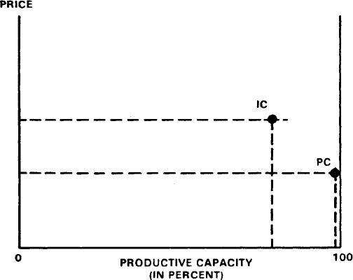
FIGURE 33:

COMPARISON OF PERFECT COMPETITION AND IMPERFECT COMPETITION

II. The Horizontal Demand Schedule

The technical textbook analysis which ends up concluding that the PC model is superior to any of the IC models runs along two related paths. One path explores the fact that the demand schedule facing the PC firm becomes horizontal, whereas the IC firm retains the familiar downward sloping D schedule. Along this path we will uncover several implications of the horizontal D curve compared with the sloping D curve. This analysis will involve elements covered in Chapters VII and VIII.

The second path is concerned with the question: Assuming both PC and IC firms seek to maximize profits, and given their respective horizontal and sloping D curves, which particular combination of P and Q will enable each firm to maximize its profits? That is to say, of all the possible dots (i.e., P and Qd) along their respective demand schedules, which one should the PC and IC firms select as the profit-maximizing one, such that any other P and Q would be less than profit-maximizing? To prepare for this particular analysis, some new technical concepts, such as “marginal cost” and “marginal revenue,” must be introduced.

From Inelastic to Elastic

How do we start to understand the horizontal demand curve of the PC firm? How does the D curve lose its downward slope from left to right and acquire a horizontal slope? Figure 34 helps us reach an answer. Imagine, first, a real-world firm with the inelastic D schedule. The dot indicates the firm’s initial position with respect to P and Q. If it raised it price, it would lose some unit sales, but because of its inelastic D its TR would increase. Other things being equal, the increased TR would leave it better off. Let us now take the next step in the analysis.

Imagine that just before our firm could take advantage of its inelastic D by raising its price, the industry is invaded by a host of new competitors from home and abroad. One consequence of this massive influx of competition and increased supply is a downward pressure on market price, as we saw in Chapter VIII. But more important for our purpose is the effect of the increased competition on the slope of our firm’s D curve. As we saw in Chapter VII, an increase in the number of firms producing similar products will tend to make D more elastic, that is, D will slope more to the horizontal, as shown by D2 in our diagram. And what a difference this makes! Let us see why.

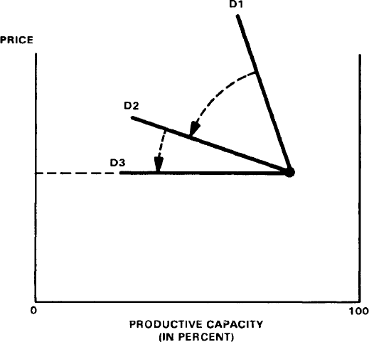
FIGURE 34:

ORIGIN OF HORIZONTAL DEMAND SCHEDULE.

Infinite Supply of Close Substitutes

Compare the new demand D2 with the former D1. First of all, D2 clearly looks elastic, which means that if our firm now dared to raise its P it would lose proportionally more unit sales than under D1, and its TR would decrease! Not only is this bad news for the firm, but it also reflects the effect of the increased availability of close substitutes caused by the huge influx of new firms producing a similar product. As we saw in Chapter VII, the greater the availability of close substitutes, the more elastic will D be. Now, let us go one step further in our analysis.

Imagine now the ultimate—that the influx of new firms into the industry continues indefinitely. Here is where we must stretch our imagination a bit: the continuous influx of new firms producing a similar product will infinitely increase the availability of close substitutes. The ultimate theoretical and graphical consequence is shown by the perfectly horizontal D3. Freedom of entry and the infinite availability of close substitutes have achieved their ultimate effect by causing perfect elasticity of D—that is, perfect horizontality in the demand schedule. We now have the explanation of the horizontal D. But our travels are not yet ended.

At this point we should note that our firm and its industry have reached the general condition characteristic of perfect competition: all firms are producing a similar, highly substitutable product (homogeneity); the number of firms has become “infinitely” great and, therefore, the size of each firm (relative to the total size of the industry) has become “infinitely” tiny (atomism); and freedom of entry has made possible the endless influx of competition. This awareness that we have reached essentially PC conditions will help us as we proceed.

No One Dares Raise His Price

We must now ask: What would happen to our firm if, faced with D3, it would again try to raise its price? How many unit sales would it lose? The perfectly flat D3 tells us. The firm would lose all of its remaining customers! Not even one unit could be sold at the above-market price! All of this can be explained: if our firm dares to raise its P, while other firms do not, no consumer would want to buy from it when he could get the same thing from its rivals at the unraised price. Given the virtually infinite number of competitors, the consumer finds it extremely convenient to buy from competitors whose unraised prices still prevail. If we simply remember the assumption of perfect knowledge, the consumer automatically knows where alternative suppliers and unraised prices are available.

In this connection it helps to emphasize that real-world firms typically face the familiar downward sloping D schedule, which looks like D1 or D2 in Figure 34. This means that if any firm dares to raise its selling P above its rival’s price, it would lose some but not all of its customers. The important thing to note is why the firm would not lose all of its customers: customers cannot find perfect substitutes for the firm’s product. Consequently, some of them continue to patronize the firm. The reason for this continued loyalty might be one of the following: customers still perceive the product as being sufficiently differentiated from rival firms’ products; or there are too many rival firms which makes it too costly to search for and locate a lower-priced source.

There is a more technical way of putting this: the horizontal D follows necessarily from the PC market structure. Product homogeneity assures perfect substitutability among products of separate firms. Unlimited competition means that each firm is necessarily a teeny atomistic entity, accounting for only an itsy-bitsy fraction of the industry output. Indeed, each PC firm is so small that it can readily sell all of its output (i.e., 100 percent of its productive capacity) at the current market price. Since consumers possess perfect knowledge, and all products are homogeneous, firms do not need to advertise or otherwise promote their product.

Meet the “Price-Taker”

In effect, all these special PC conditions cause the PC firm to end up as a totally passive, submissive agent—a mere price-taker, as some writers put it—obediently accepting the market price as its own selling price. Our new Figure 35 helps us see this connection between the PC firm as price-taker and the horizontality of its demand schedule, as it perceives it. In panel A, the market dishes up a market-clearing price based on the momentary D and S conditions. Then, somehow, by some magical mystery device, the market automatically transmits information about this price to every firm, as shown by the arrow pointing to panel B. Panel B shows the firm “taking” the market price, adopting it as its own selling price, at which price it can then sell as much as it wants to produce.

In other words, the horizontal D schedule facing each price-taker is merely saying to the firm: the market says there is only one price at which you can sell your current product, and this is it; there is no sense in trying to sell at any other price. For instance, if you set your price above the market price, you will lose all sales to your rivals. On the other hand, there is no point selling below the market price since the market says you can sell all you want at the (higher) market price. Thus, the horizontal D schedule is essentially a price line in the same way that the familiar downward-sloping demand schedule constitutes a “price line”: all demand schedules, regardless of degree of slope, indicate the price at which a given quantity can be sold to demanders.

A Possible Confusion

In this connection, let us anticipate a question concerning the apparent conflict between the traditional downward-sloping market demand schedule and the perfectly horizontal demand schedule facing the individual firm under PC. Actually, there is no real conflict: the horizontal D is an abstraction related to an unreal PC model, and hence is an impossibility, whereas the downward-sloping market D is a real-world concept. Market demand schedules will always have the familiar downward slope (remember Chapter VI). As for the demand schedule facing the individual firm in the real world, it too will possess varying degrees of downward slope so long as its product is differentiated and the number of rival firms is more or less limited (see Chapter VII on elasticity of demand). In contrast, the horizontal D schedule is merely the logical outcome of extreme conditions postulated by the PC model: absence of product differentiation and unlimited number of rival firms.

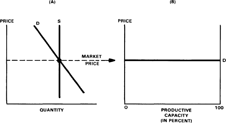
FIGURE 35:

PRICE-TAKER’S HORIZONTAL DEMAND SCHEDULE.

III. Profit Maximization: MC vs. MR

We have reached the half-way point on our trek to discover the secret of Figure 33: why the perfect competition (PC) firm is alleged to produce more and sell at a lower price than the imperfect competition (IC) firm. On the first leg of our journey we explored the nature and implications of the horizontal demand schedule. We now explore the method by which firms are supposed to maximize profits, that is, the “marginal cost” versus “marginal revenue” method. In order to understand this rather technical approach to profit-maximization, we must first explain the concepts of marginal costs (MC) and marginal revenue (MR).

Costs, Fixed and Variable

The concept of marginal costs (MC) is simply derived from the concept of total costs (TC). As the term indicates, TC includes all current and capital expenses incurred by the firm in production. Generally speaking, the higher the rate of production—that is, the higher the rate of productive capacity utilized—the larger is TC.

Textbooks distinguish two main components of TC: “fixed costs” (FC) and “variable costs” (VC). Again, the terms indicate their respective meanings. Those costs which are classified as fixed costs are so called because, by their nature, they remain fixed or unchanged in total dollars regardless of the firm’s rate of output. The other costs, which are classified as variable costs, are so called for the opposite reason—they do not remain the same but, rather, vary in amount according to the different rates of output. These general characteristics of the TC, FC, and VC schedules are shown in Figure 36, panel A.

Leading examples of FC—which textbooks also call “overhead” or “sunk” costs—are rent, depreciation, property taxes, and salaries of overhead personnel (e.g., executives, department chiefs). Leading examples of VC are wages of direct labor, materials, water, and electricity.

We can now see in Figure 36 why TC rises as the rate of output increases: it is due to the VC component, since FC remains constant. The reasons for this characteristic behavior of VC are several: the increase in output generally requires more inputs of labor, materials, and power. However, at the highest rates of output (say, 85-100 percent of capacity) premium rates of pay for overtime labor may be incurred; overtime operations are regarded as less efficient than day-shift operations; any additional workers hired may be less efficient than the regular labor force, thereby causing an increase in unit costs of output; and continuous high rates of plant utilization often cause equipment breakdowns and expenses for repair.

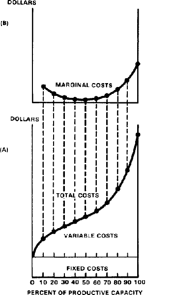
FIGURE 36:

TOTAL COSTS AND MARGINAL COSTS.

Classification of Costs

How does one determine whether a given production outlay should be classified as “fixed” or “variable”? Theoretically, it is very simple: it depends on whether the dollar outlays for the given expense item are affected by, and vary with, the rate of output. If they vary whenever the rate of output varies, it is a variable cost. Otherwise, if they stay the same in dollar amount, regardless of the rate of output, it is a fixed cost. In practice, however, the accounting for such expense allocation may be more complicated than in principle.

The reader should be alerted to the fact that Figure 36 depicts a typically short-run situation. The “short-run” is defined as that time period during which the productive capacity of the firm is presumed to be fixed, unchanged. In our analysis, whenever we refer to “productive capacity,” we are assuming a given, short-run situation during which plant, equipment, and other overhead items remain the same; the only things that vary in the short run are the variable expense items, such as labor and materials.

From TC to MC

It is from TC that we derive the marginal costs (MC) in a straightforward way. First, MC is defined as the increment of increase (or decrease) in TC when production is increased (or decreased) by one unit of output. For instance, if an increase in output of one unit increases TC from $1,200 to $1,300, then the MC is $100, the increment of increase in TC.

Although Figure 36 is drawn in terms of rates of output (e.g., increments of 10% each of productive capacity), and not in terms of single units of output (e.g., one ton of coal), the principle of derivation remains the same, as shown in panel B. By extracting the increments of change in TC from panel A and connecting their heights in panel B, we are able to derive a characteristic MC curve. Indeed, the MC schedule turns out to be a reflection of the incremental changes in VC as well as TC. The reason for this, as we saw above, is that the marginal changes in VC account for the marginal changes in TC to start with.

From TR to MR

Derivation of the marginal revenue (MR) schedule of the firm is less complicated. Indeed, all we need to start is a demand schedule: an array of prices (P) and the quantity demanded (Qd) at each respective P. This D schedule enables us to derive total revenue (TR); and it is this TR from which marginal revenue is derived in the same incremental way as MC is derived from TC.

The following Table VI (A) illustrates the simple arithmetic involved. When P is reduced, Qd increases and, in this case, so does TR. MR, in this case, is the extra revenue from selling an additional unit. Thus, as TR increases from $1,000 to $1,089, MR amounts to $89, and so on. Indeed, MR can be defined simply as the increment of change in TR when one more—or one less—unit is sold.

“Spoiling the Market”

Notice the following characteristics of the TR and MR schedules derived from the D schedule in Table VI (A). First, for all downward-sloping schedules, so long as the TR schedule increases when P is reduced (i.e., D is elastic), it increases at a diminishing rate—by diminished increments—as seen in the MR column: MR decreases even though TR increases.

The diminishing rate of growth in the TR, and hence the MR, is itself a consequence of the “spoiling-of-the-market” effect that naturally occurs when firms reduce their P in order to increase the number of units sold. Since the lower P is applied to all units offered for sale, the firm necessarily takes a beating, so to speak. For example, in order to sell 11 units instead of 10, the firm must reduce its P for all 11 units. This differs from the practice called multi-part pricing, under which the firm would sell the first 10 units at the original $100 and then sell only the 11th unit at $99, the 12th unit at $98, and so on. Instead, the firm applies the new, lower P to all units sold, and not merely to a part of them.

TABLE VI

(A) Marginal Revenue—Sloping D

Price(p)	Quantity Demanded (Qd)	Total Revenue (TR)	Marginal Revenue (MR)
$100	10	$1,000	$—
99	11	1,089	89
98	12	1,176	87
97	13	1,261	85
96	14	1,344	83
95	15	1,425	81
94	16	1,504	79

(B) Marginal Revenue—Horizontal D

Price (P)	Quantity Demanded (Qd)	Total Revenue (TR)	Marginal Revenue (MR)
$100	1	$100	$—
100	2	200	100
100	3	300	100
100	4	400	100
100	5	500	100
100	6	600	100
100	7	700	100

This brings us to an important associated characteristic of the MR for a downward sloping D: at every selling P, the MR is less than the corresponding P. This, too, can be seen in Table VI (A): at a P of $99, MR is only $89; at a P of $98, the MR is only $87; and so on. This characteristic tendency is likewise attributed to TR growing at a diminishing rate when D is elastic, that is, the “spoiling-of-the-market” effect noted above. We can graphically illustrate these characteristic features of MR in its relation to TR in Figure 37, panel A.

MR for the Horizontal D

So far, our discussion of the MR schedule is relevant only to the case of imperfect competition (IC), not to perfect competition (PC). The reason is that only in IC do we find downward-sloping demand schedules which do not exist in PC, where D schedules are necessarily horizontal. Under IC, demand schedules facing the firm characteristically slope downward because of product differentiation, as we saw in our discussion of Figure 34.

Mathematically, the MR derived from a horizontal D is calculated in the same way as for a sloping D (see Table VI (B)). But whereas MR is always less than P in the case of the sloping D, MR is always equal to P in the case of horizontal D schedules. For every unit sold there is only one P, the market P. Thus, since the horizontal D of the PC firm is its “price line,” it is also its MR schedule. This characteristic coincidence of MR and P under perfect competition is illustrated by the P and MR schedules in Table VI (B) and in Figure 37, panel B.

Determining Maximum-Profit P and Q

We now approach the climax of the textbook case in favor of the PC firm and against the IC firm. At this stage of the analysis both types of firms are asked to determine their maximum-profit price and quantity by means of “marrying,” so to speak, their respective MC and MR schedules. That is to say, they are both asked to apply a special method of determining that unique P and Q combination at which total profits will be a maximum, such that any other P and Q would yield less than maximum total profits. At its heart this method involves the juxtaposition of the MC and MR schedules relevant to the PC and IC firms, respectively. Let us first examine the case of the PC firm.

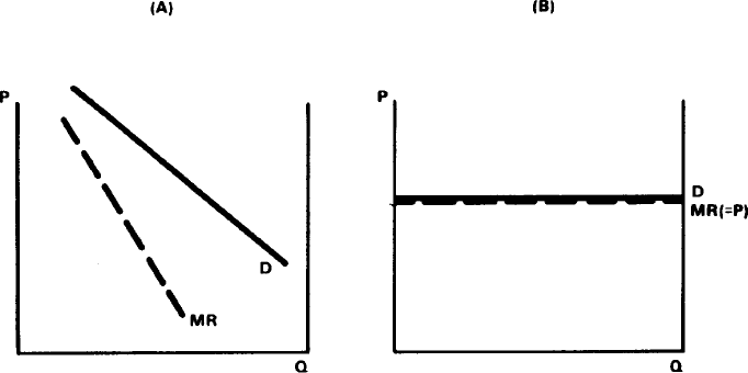
FIGURE 37:

MARGINAL REVENUE CURVES

How the Price-Taker Maximizes

How does the atomistic price-taker in PC determine his maximum-profit P and Q? According to the textbooks, we must look for that unique combination of P and Q at which MC equals MR—that is, graphically speaking, the intersection point of MC with MR. This special meeting place of MC and MR points out that particular price (P) and output (Q) which will maximize the firm’s profits. This intersection point, where MC equals MR, is readily seen in Figure 38, panel A: it points both to the P (i.e., $100) along the horizontal D, and to the Q (vertically downwards, the quantity X). (Remember, for the price-taker and his horizontal D, the market P represents his MR, too). In this case, then, a P of $100 and a Q amounting to X are the unique pair of P and Q that maximizes total profits. Any other P and Q would be less than maximizing under the given MC and MR conditions. Why? Let us see.

A simple, logical process of elimination enables us to see why only that pair of P and Q at which MC equals MR brings maximum profits. If we look at panel A in Figure 38, we notice that the market has already given our price-taker the price at which he must sell; it remains for him only to find that unique quantity which will maximize his total profits. And we find this special Q at the output X that is indicated by the intersection point of MC with MR: only output X can maximize total profits; any other Q will bring less than maximum profits.

For example, if the price-taker produces more than X, MC will increase and exceed MR; this means that the extra costs of producing the additional units would be greater than the extra sales revenue and would, therefore, detract from total profits. Conversely, if the firm produces less than X, the MC is being exceeded by the MR, which means that the firm can still add to its total profits by producing more. Only when it reaches output X will the firm discover that its MC has finally caught up with its MR so that no more profits can be added by producing still more.

Balancing Costs vs. Benefits

To put it another way: it always pays the price-taker to produce more so long as MR exceeds MC, and to produce less when MR is exceeded by MC. That is to say, so long as MR is greater than MC, additional profits can be earned by producing more, even though MC is continuing to rise: this rise in MC is merely slowing down the increments of increase in total profits but is not stopping total profits from growing. (Indeed, total profits continue to increase, albeit at a diminishing rate.) Similarly, so long as MR is being exceeded by MC, it means that the hitherto earned batch of profits is being eaten up by the excess of MC over MR. This excess of MC over MR is the signal that the firm is producing too much.

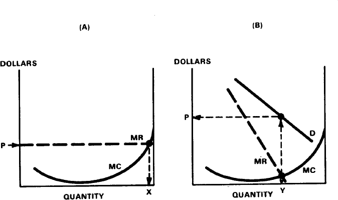
FIGURE 38:

PROFIT MAXIMIZATION

Actually, this principle by which the firm balances MR against MC is merely a special case of a general principle: It pays to put out extra effort or sacrifice (MC) so long as the extra benefits or gain (MR) exceeds it. The only difference between the application of this principle to (a) the firm, and to (b) human action in general, is that in the former case it is easier to quantify or assign numerical values to MC and MR, whereas in the latter case it is not possible to quantify the subjective valuations attached to extra sacrifices and extra benefits.

Price-Taker Is a Quantity Adjuster

At this point it is relevant to note that the PC firm is not only a price-taker but is also a quantity-adjuster. That is to say, once he is given the market P, he need only adjust his quantity of output to that rate which is indicated by the intersection of MC and MR and which will, therefore, maximize his profits.

For example, if on a given day the market price rises—say, from P1 to P2 in Figure 39—this causes a rise in marginal revenue schedule from MR1 to MR2 and a new intersection point with the unchanged MC schedule. This in turn indicates a new (higher) rate of output (to Y) that would maximize profits. Conversely, if the market price decreases—say, from P1 to P3—the new intersection point of MR with MC indicates a reduction in output to the rate of Z. In summary, rising market prices enable output to expand into the higher MC ranges, whereas falling prices drive output down into lower MC ranges.

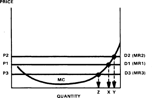
FIGURE 39:

PRICE-TAKER AS QUANTITY-ADJUSTER.

How IC Firms Maximize Profits

In contrast to the price-taker in the PC model, how does the firm in the IC market structure—monopoly, oligopoly, or monopolistic competition—maximize its profits? In the textbooks, the answer is straightforward: apply the same profit-maximizing principle. That is, look for the intersection of MC with MR, since only that P and Q which make MC and MR equal can maximize profits. Precisely this has been done in Figure 38, panel B. But notice some differences due to the sloping demand schedule characteristic of IC firms, to wit.

The downward-sloping demand schedule of the IC firm as we saw in Figure 37, panel A, generates a still greater downward slope in the MR schedule. For this reason we get a different intersection point for MC and MR, even though the MC schedule is the same in both cases: The intersection will characteristically occur at a point that is lower and leftward along the MC curve (see Figure 38). It is from this differently located junction of MC and MR that we now read off that unique P and Q combination that maximizes profits for the IC firm. When we do this, we find that the MC:MR intersection points to the smaller output of Y and the higher price than in panel A (remember, price is always read off the demand schedule).

Voilà! Less Q, Higher P

It is here that we have the textbook answer to our original conundrum—that the atomistic price-taker characteristically produces more and at a lower price compared to the IC firm whose Q is typically smaller and its P higher. Ostensibly, the key to the puzzle is the downward slope of the demand schedule characteristic of the IC market structure! If only the IC firm were not facing a sloping D schedule—that is, if it instead had a horizontal D curve—it, too, would produce as much as the PC firm and at as low a price. Only the sloping D induces it to retreat to the smaller Q and the higher P for its maximum profits; any lower P and greater Q would only cause a drop in total profits. Let us now proceed to raise a sticky question: To what extent is the sloping D really the key to the puzzle?

IV. Taking Stock of “Perfect Competition”

How are we to evaluate this textbook case in favor of the PC model? First, we will examine the PC model on its own terms to see if it really holds up as a superior model of competition. How realistic is “perfect competition” as a model or standard for real-world competition? How desirable is the PC model, even if it were possible to implement? Then we will swing over to the IC model and see if things there are really as inferior as they are made out to be. Let us now briefly review the realism of the four basic assumptions underlying the PC model.

Is Perfect Competition Realistic?

It should be clear by now that the PC model starts right off with three strikes against it by assuming the triad of product homogeneity, atomism of firm size, and perfect knowledge. All three are patently unrealistic conditions, yet the PC model brushes this handicap under the rug. It is like saying a person could fly merely by assuming that he already had wings! How does one get wings in the first place? How do we achieve homogeneity, atomism, and omniscience to start with?

Illusions of Perfect Knowledge

Omniscience? Perfect knowledge? How does this apply to real life? Knowledge or information are scarce resources because the means of acquiring them, and of overcoming ignorance in general, are themselves scarce and therefore costly to acquire: the time, effort, and money required for searching, trial-and-error experience, and learning.

Worst of all, the world does not stand still—it is in constant flux; demand schedules shift, techniques of production become obsolete through the introduction of new and better ones, and the supply and quality of resources alternately worsen or improve. The result is constant change in demand, supply, and prices—change that makes them unpredictable. As soon as we learn a given fact, so soon is it likely to become obsolete. At best we can expect only to acquire that amount of information which will hopefully maximize the likelihood of non-regretful decisions. For everyone to possess perfect knowledge, however, you would have to make the world stand still and remain changeless until everyone could obtain all the information he needed to make non-regretful decisions. That is, only in a static world would perfect knowledge be possible.

Homogeneity vs. Nature

Homogeneity of product? This goes entirely against the natural tendency of human beings to differentiate and distinguish themselves simply because they are differentiated by birth. Whether it is by creating different products or rendering individuated services, each of us naturally seeks to individualize his personality and talents in some self-satisfying way. Hence, it is unreasonable to expect differentiated human beings to produce naturally a flow of undifferentiated (homogeneous) goods and services. The only way you can get homogeneity of product is first to produce homogeneous people. Short of that, you would have to impose a dictatorship to compel people to produce homogeneous results.

Atomism vs. Productivity

How about atomism of firm size? Theoretically, the smallest irreducible size of the firm is the individual producer, working on his own homestead. Offhand, it is difficult to object per se to such individual farmers, craftsmen, industrial artisans, and self-employed professionals as the basis of a household economy. But an individualist economy does not necessarily imply homogeneity of product instead of differentiation. Indeed, given the natural tendency for human differentiation, it is more reasonable to expect differentiation rather than homogeneity of product in a household economy!

Furthermore, history tells us that, when given the chance, man would just as soon give up his household economy and participate in the social division of labor in order to enjoy its multitude of benefits: the economies of large-scale production and their associated lower costs and prices, the greater supply of human talents that can be pooled in one locale, and the greater variety of goods and services available in one market. Again, the only way you might get a universal reversion to one-man household economies would be by totalitarian force.

An Inner Inconsistency

This brings us to an embarrasing inconsistency immanent in the PC assumptions—specifically, between atomism and homogeneity. It can be argued that the two key requirements of homogeneity and atomism are not necessarily mutually compatible. Thus, it does not necessarily follow that product homogeneity is more compatible with endless numbers of atomistic firms than is product differentiation. Indeed, on the basis of both logic and history, quite the contrary can be argued: It is standardization of product that could reasonably be associated with massive concentration of production within a few giant firms (i.e., oligopoly), whereas differentiation of product would naturally be associated with the host of atomistically small, independent producers, each turning out his more-or-less individualized product.

For one thing, standardized products are technically more easily adapted to large-scale mass production methods. (The Industrial Revolution proved that.) Add to this the economic attraction of lower unit costs and prices permitted by large-scale production. Hence, there is the undoubted attraction of concentrating production in a relatively few large-scale plants. In contrast, differentiation of product necessarily implies separate small plants or workships for each separate craftsman; and since there is no conceivable limit to the number of different products man can create, there is no assignable limit to the number of firms or workshops that would be established, except the limit posed by scarcity of resources. Thus, atomism does not necessarily mean homogeneity of product; the PC model is stood on its head.

Free Entry Makes Sense

What’s left? It’s free entry—freedom to compete—at last something we can accept as a reasonable way to achieve maximum production and exchange, and hence maximum consumers’ welfare. But, as we saw in Chapter X (on consumers’ sovereignty), the free-market system also features freedom of entry. Why push for fantastic perfect competition, with its triple chimera of homogeneity, atomism, and perfect knowledge? If free entry is desirable, then the free-market model would seem to be a more reasonable objective than impossible PC.

No Real Competition in PC!

This brings us to another serious flaw in PC. Where, oh where, is there any real competition in this “perfectly competitive” model? Where is there even a whiff of rivalrous behavior in this world of passive quantity-adjusters? For example, where is there any price competition? As a matter of fact, the PC model precludes any incentive to engage in competitive pricing since each price-taker is a mere quantity-adjuster. Where is there any non-price or quality competition through product differentiation? There is none of that, either; it is homogeneity which rules the roost. The only rivalrous dimension in the whole of PC is free entry. But as we have just seen, free entry is by no means unique to the PC model. More important, however, free entry under PC becomes a meaningless feature: Firms are free to enter into only passive, noncompetitive production as mere quantity-adjusters! So again it must be asked: Where is there any real competition in PC?

This is a real embarrassment! After all, how can anyone sensibly hold PC up as a model of competition when, by definition, it is totally barren of any real competition for the consumer’s dollar? Thus, the free-entry condition provides only a delusive dimension of rivalry: PC firms are free to produce only homogeneous products. Indeed, as we will soon see, every attempt to compete by means of product differentiation or cost-cutting innovations proves to be futile—which is enough to kill off any incentive to compete in the first place. We will now see why.

Competition in the Real World

In the real world, as distinguished from the passive world of PC, competition only superficially takes place in terms of lower price and better quality. Underlying both price and quality competition is innovation—those seminal activities that bring about (a) the product differentiation that enables the conquering of markets, and (b) the cost-cutting that enables firms to reduce prices without squeezing profit margins (see Chapter IV). Indeed, we will now see why only in the real world would it be reasonable to expect such innovation to occur, and why it is unreasonable to expect any innovation under PC.

By means of product differentiation, firms seek to tap new markets by filling gaps in market demand—demand to satisfy wants or demand for new means. As long as people’s tastes blossom and develop in endless variety and sophistication, and as long as people are naturally inclined to keep up with the Joneses, the market will continue to reveal “gaps” of unsatisfied demand which entrepreneurs will seek to fill. But none of this will happen automatically: only the alert firms, and the ones that command sufficient capital funds, will be able to capitalize on the untapped gaps in market demand.

Instantaneous Imitation of Product

In contrast, the PC model offers only homogeneity of product. We must now ask: What would happen in PC if a maverick firm, having spotted an untapped gap in market demand, decides to innovate—by producing a new product, improving on an existing one, or modifying it with a new style or design? Such innovation could enable this firm to increase it sales, grow in size, and increase its share of the market. However, given the magical assumptions of PC, such advantages would be extremely short-lived: perfect knowledge, mobile factors of production, and the firms’ ability to instantaneously imitate any innovation would immediately erase any advantage to the innovator. Right on the heels of the innovator, all other firms would instantaneously duplicate the innovator’s feat in order to recoup their lost shares of the market. As a consequence, innovators would soon realize that, given the likelihood of instantaneous imitation by rivals, it would be utterly foolish to innovate in the first place. Why bother?!

We can now also see why the PC model, which precludes product differentiation, is so unreal. In the real world it would take at least some time before any or all rivals could catch up with the innovator: resources are not so mobile as in PC; nor does every firm have personnel as talented or creative as the innovator’s. Indeed, we can now see that the PC assumption of instantaneous imitation implies that every firm has equally talented personnel. Only this equality assures that what any one PC firm can do, every other firm can do as well, and instantaneously. In PC, homogeneity of product implies homogeneity of personnel!

Instantaneous Imitation of Technique

A similar threat of instantaneous duplication by rivals hangs over the PC firm if it dares to innovate new cost-cutting techniques. Why on earth would a firm introduce a new technique of production in the first place if rival firms can duplicate this feat in a jiffy? We can now see the real reason why, when faced with a horizontal D schedule, it would be foolish for the firm to sell below the market price. The reason is not simply that the firm is taking the easy way out by passively “taking” the market price; it is a bit more complicated than that.

First of all, selling below the market price means that, as a result of its price-cut, the firm’s profit margin will be squeezed. True, this underpricing of product is silly if you are in PC and you are free to “take” the higher market price and still be able to sell all that you produce. So long as you are motivated to maximize your profits and wealth, so long will you prefer to sell at a higher price than at a lower price, ceteris paribus. Therefore, it makes no sense to squeeze your profit margin if you don’t have to. But what if you can introduce a cost-cutting technique and cut your selling price without squeezing the profit margin? And what if you alone are able to cut costs while your rivals cannot, so that you can cut your price without cutting your profit rate while your rivals cannot do so? This possibility is diagrammed in Figure 40.

Unit Cost or AC Schedule

The first thing to note in Figure 40 is the average cost (AC) curve introduced in panel B. Based on observed date, the AC schedule shows the varied cost-per-unit of output incurred at different rates of production. At very low rates of production—say, in the OX range—the AC is above the minimum unit costs that occur in the large XY range of productive capacity. Only when the plant is operating at these higher rates of capacity—in the XY range—can it enjoy the minimum unit costs. Then, at the very high rates of production, in the approximately 85-100 percent of capacity range (YZ), unit costs again rise above minimum costs. The reasons for this are several-fold: overtime rates of pay; costs of repair and maintenance of overburdened equipment; and drop in productivity due to newly hired workers.

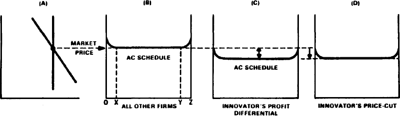
FIGURE 40:

INNOVATIVE COST-CUTTING AND PROFIT DIFFERENTIALS.

The next thing to note in panel B of Figure 40 is that the current market price just covers the minimum points of the AC curve. Since textbooks usually include a “normal” rate of profit in the AC schedule, this means that firms are able to earn a normal profit when their AC is covered by the going market price. (The reader should be aware that this inclusion of profit in the AC schedule differs from the treatment in Chapter IX. This difference of treatment is still an unresolved question in the technical literature. Here we adhere to the orthodox treatment, unless otherwise specified.)

This tangency of market price and minimum AC represents a state of equilibrium. If market price were to fall below AC, losses would begin to replace profits, firms would begin to exit from the industry, and the reduced supply would tend to drive prices back up again. The restored price level would then make it once again profitable to enter the industry. If, on the other hand, prices were to rise above the original level, the extra profits would attract new firms whose entry would increase supply and drive prices back down, thus reducing profits to their former rate.

Source of Differential Profits

Now, in panel C we can see the initial positive impact on the innovator’s profits of his newly introduced cost-cutting technique. The new technique of production enables the innovator’s AC schedule to drop; this means a lower unit cost of production. Since market price is still the same as before, the innovator’s lower AC automatically increases the spread between selling price and AC. Thus our cost-cutting innovator enjoys initial differential profits—a higher profit rate than his rivals’.

He now has two basic choices: (a) continue to enjoy the full margin of differential profits, while leaving his selling price the same as his rivals’ (panel C); or (b) reduce his selling price to where it just covers his minimum AC (panel D). The first option would generate an accumulation of profits and increase his wealth, while the second option could enable him to underprice his rivals and drive them out of business. (A very important byproduct of this rivalry between our innovator and the laggards is the lower price enjoyed by consumers). Since his rivals cannot match his lower price without suffering drastic losses, they lose customers to the innovator. But then our innovator would have to expand his productive capacity in order to supply the increased demand for his product.

Whence will our innovator obtain additional funds to invest in new plant and equipment? He can, of course, borrow from the money and capital markets; but he now also has a new source of investment funds: the differential profits associated with choice (a) above. However, the innovator, in line with much of U.S. experience, could decide upon a combination of both (a) and (b), enjoying part of the financial benefits accruing from (a) and part of the competitive benefits accruing from (b).

Instantaneous vs. Delayed Ajustments

Whichever course our innovator undertakes as a consequence of his initial differential profits, the fact remains that these profits can arise only so long as none or very few of his rivals can duplicate his cost-cutting feat, and so long as there is a sufficient time-lag between his innovative advance and his rivals’ catching up to him. In real-world competition, significant differential profits are possible precisely because firms are not equally capable of innovative advances and cannot instantaneously imitate the innovator’s feat. In the PC model, however, all firms are required to be equally capable in every dimension of competitive behavior. Ironically, as a consequence, no real-world competition would actually take place. Why compete when there is no advantage to it?

In the real world, by contrast, firms do have incentive to innovate precisely because the inequality of talents and creativity, on the one hand, and the time-lags involved in catching up to the innovator, on the other, may be sufficient to bring pioneer profits to firms able to innovate. By the same token, the laggard firms, in order to catch up, are desperately driven to at least imitate the innovator, if not to innovate on their own. Otherwise, they must resign themselves to a secondary position in the industry. In the process of imitation, the imitating firms may resort to luring away key personnel from the innovator, intensive market research, product planning, and research and development. Such catch-up efforts thus give an ironic twist to real -world rivalry among firms: to the extent that laggards intensify their imitation of the innovator—for example, in style or design—to that extent a tendency to homogeneity asserts itself and offsets the tendency to differentiate products.

Homogeneity of Firms, Too

All of this helps bring home another important implication of the PC model already noted above: The logical concomitant of homogeneity of product is the homogeneity of firms! The personnel of firms themselves must be as homogeneous as the products they produce. The talents embodied in each firm must be equally knowledgeable and creative in order to be able to achieve instantaneous imitation of a rival’s innovation. It is as though the goddess of egalitarianism had descended upon the world and redistributed the differentiated talents of the world in order to create an even distribution of them. Hence the motto, “Anything you can do, we can do!” appropriately describes what homogeneity of product in PC really implies.

Is Perfect Competition Desirable?

Let us grant that no one really wants a reincarnation of the PC model under real-world conditions, and that proponents of the PC model merely want us to approximate it—by promoting tendencies toward homogeneity, atomism, perfect knowledge, and free entry. After all, aren’t these, in themselves, desirable characteristics for a competitive economy?

Well, to start, what about the desirability of homogeneity? This characteristic must be ruled out simply on the logical grounds that it makes no sense to desire something that either (a) is impossible to achieve (given the axiom of human differentiation) or (b) is achievable only by undesirable means (i.e., totalitarianism). Atomism of firms must be disqualified on virtually the same grounds. Furthermore, as we have argued, atomism is more compatible with product differentiation than with homogeneity.

Perfect knowledge, too, must be rejected on the grounds of impossibility. This is not to imply the people will not prefer more knowledge to less knowledge, but only that personal circumstances and subjective preferences of each individual—the degree of urgency and motivation, and the availability of means—can determine the extent to which a person pursues greater knowledge.

Finally, we are again left with free entry as the only realistic and the only desirable goal in PC. We have already noted that free entry implies essentially the same thing as free competition in the free-market model in Chapter X: the absence of artificial barriers to new or existing firms that want to enter into competition in the given industry. But, as we have stressed, free entry is the only realistic element in PC; the rest of it—homogeneity, atomism, and perfect knowledge—must be abandoned as unrealistic goals.

Free Entry Means Free Market

If free competition is the most we can ask for in the real world, and the free market assures maximum free competition, it is reasonable to ask: Why bother with the impossible PC model when the free-market model—which is not impossible!—will suffice? Why saddle ourselves with the chimera of product homogeneity, atomistic firms, and perfect knowledge if the only necessary condition is free-market competition?

To repeat: the only one of the four basic assumptions of the PC model that can serve as a real-world starting point for creating more elastic D schedules is free entry; the only thing it requires is the removal of artificial impediments to free competition. In contrast, the other three assumptions cannot serve as starting points because they are impossible; nor can they serve as end results because they are either beyond human capability (e.g., perfect knowledge) or desirability(e.g., homogeneity, atomism).

Sloping Demand the Achilles’ Heel

Let us now swing back to the much discredited IC firm, which is alleged to produce less Q at a higher P than the PC firm, and therefore is regarded less satisfactory than the imaginary PC firm. What is the single apparent cause of this inferiority? Technically speaking, as noted above, it is the sloping demand schedule. Everything else in the textbook argument seems OK—that is, since the marginal cost schedule is assumed to be the same as that of the PC firm, the Achilles’ heel must be the sloping D.

If the sloping demand schedule automatically condemns the IC firm, it is proper to ask: What causes this slope in the first place? The answer is: product differentiation—the absence of very close substitutes. This even includes monopoly—open or closed—since its being the only firm in its field naturally differentiates it from all firms. Except for the closed monopoly, however, differentiation of product is, as we have noted, a byproduct of the natural differentiation of human beings—consumers having varied tastes and preference-scales, and producers having differentiated ability to cater to consumers’ wants. Thus the indictment of the IC firm basically implies a denial of natural human variation—as though demand schedules in the real world could be anything but sloping!

Producing Less for a Higher Price

Is there any way of saving the IC firm from the curse of its sloping demand schedule, which alone induces it to produce a smaller Q at a higher P? One obvious way out would seem to be this: Let the firm settle for less than maximum profits! That is to say, let it produce more Q and sell at a lower P; for example, more than the amount Y in Figure 38, panel B; then drop the P in order to sell this greater Q. But this raises the obvious question: Why should the IC firm be forced to seek less than maximum profits? Does it not have the same right as the atomistic PC firm to seek maximum profits? It certainly does—but only by means of producing less and selling at a higher P. This question, in turn, brings up the more fundamental issue: Does not every firm have the right to produce as much or as little as it wishes?

For example, does Clint Eastwood have the right to ask for a higher salary than, say, Robert Redford—or vice versa? Does either of them have the right to make only one picture a year, if he wishes, instead of two or three? Does anyone have the right to compel them to make more movies for less pay per movie? Does the farmer have the right to sell less corn at a higher price per ear? Does the electrical worker have the right to ask for a shorter work week and a higher rate of pay per hour? Is there anyone working a forty-hour week who cannot be accused of preferring this to working fifty hours at less per hour?

Common law tradition has it that everyone has the natural right to produce as much or as little as he wishes, which includes working a shorter work week while asking for a higher price for his service. But he does not have the right—at least in a truly free society, with individual rights of self-sovereignty—to force others to pay a higher price for less work. Unfortunately, this principle is being widely violated; leading examples are (a) trade-union strike actions to reduce working hours and increase wage rates, and (b) legally enforced farm acreage restrictions to reduce supply for higher farm prices.

Bogey of “Artificial Scarcity”

The less-Q, higher-P indictment of the IC firm is part of a general line of attack which holds that any firm that dares to produce less Q than it can is guilty of “contriving artificial scarcity.” This makes no more sense than to say that any of us who dares to rest from work or even sleep too much would also be guilty of “contriving artificial scarcity” by being less productive than otherwise.

More seriously, however, we need only recall that scarcity is a natural condition that is prior to man’s productivity. Anything useful that man produces, no matter how great or small, can only help alleviate the scarcity of goods; it certainly cannot create “artificial” scarcity! It is totally irrelevant, therefore, that an oligopolist or any other real-world firm can produce more than they do: so long as they produce anything at all, they reduce scarcity, not create it! Yes, there is a way to create artificial scarcity, and that is to forcibly prevent or restrain a person from producing goods—for instance, by artificial legal barriers to entry of the type discussed in Chapter X (e.g., licenses or permits required by government), threats and violence by a Mafia gang, by trade union and agricultural restrictionism, as noted above.

If we grant the IC firm every free man’s right to produce as much or as little as it wishes, and to charge whatever price it feels its product is worth (or whatever price the buyer is willing to pay), we must then ask: What grounds do proponents of the PC model really have for condemning the IC firm? If the IC firm does have the natural right to maximize its profits and to produce less Q at a higher P, on what grounds can we reject the IC firm?

Bogey of “Market Power”

A favorite ploy of opponents of the IC firm is the bugbear about “market power.” What is this market power? In essence, it refers to one of two things: (a) the IC firm’s ability to raise its price without fear of losing all its customers, a fear that haunts the price-taker under PC; (b) the ability of large companies to “administer prices.” In the first case, “market power” merely refers to possession of a sloping D! Only a sloping D enables the firm to hold onto some of its customers even when it raises its P. Presumably, sloping D schedules must be outlawed! But enough has already been said about sloping D curves versus horizontal ones. Let us, instead, move on to the concept of “administered prices.”

What Are “Administered Prices”?

The concept of “administered prices” (AP hereafter) implies that the large firm has an unrivaled power to raise its P at will—presumably in virtual defiance of the law of demand and supply! That is to say, the mere posting of its selling price by the firm suffices to realize this price in the market place. In the past 30 years or so, the concept of AP has cropped up whenever the general price level in the economy spurted upward—in association with charges that the big corporations were to blame for “too high” prices and “inflation.”

This is not the place to get into the true causes of price inflation. Suffice it to note that, other things being equal, the primary inducement to raising the firm’s P is to increase its TR (not decrease it). This implies that the firm believes it has an inelastic D schedule (Chapter VII): only an inelastic D will enable the firm to increase its TR by a price hike. That is, if the firm had an elastic D instead, the price hike would only cause its TR to drop and it would therefore have to rescind its price hike.

All Firms Are Price-Takers!

Two conclusions follow. One is that the bugbear about AP can only have relevance to firms possessing inelastic rather than elastic D schedules. The issue then becomes this: Does the big firm—or any firm—have the natural right to raise its P in order to increase its TR? We have argued the affirmative. More important is the second conclusion: After all is said and done, in the real world all firms turn out to be price-takers no less effectively than in the PC model.

For instance, no real-world firm really has the “power” to suspend the law of demand and supply—that is, to avoid ending up with a surplus for overpricing its product, or to avoid less-than-maximum profits by underpricing its product and realizing a shortage. Sooner or later, after trial-and-error searching for the market-clearing price, every real-world firm finds itself eventually having to “take” the market price that actually clears its supply. Thus real-world firms are “price-takers” no less than firms in pure competition, the only difference being this: PC firms “take” their P from the market right from the start (they have perfect knowledge!), whereas real firms “take” their P only after trial-and-error search in the market. Irony of ironies: real firms are, in an ultimate sense, price-takers, too!

What Firms Can or Cannot Do

To be sure, in the real world every firm is free to sell or not to sell at the going market price. For example, it is free to withhold some of its product if it believes this will cause a shortage and a rise in market price. But this “power” to withhold supply can in no way force the buyer to pay that higher price. The buyer is always free not to buy if he thinks the price is too high. The only “power” possessed by any firm is the right to post its selling price—merely to ask for whatever price it wants—that’s all! In no way can it compel any buyer to pay that price.

Thus we see that so long as the firm: (a) must seek the market-clearing price in order to avoid overpricing or underpricing its product and to maximize its profits, and (b) does not have the power to force buyers to pay its asking price, then so long must the firm—even the ugly “giant” oligopolist—be viewed as a price-taker rather than a price-controller. So long as the market demand can upset any price posted by the firm, we must conclude that it is market demand and not the firm that ultimately determines selling prices. In the absence of perfect knowledge, real-world price-takers have to grope and search for their profit-maximizing price instead of getting it automatically and instantaneously as in the unreal world of pure competition. In the real world, there is no way for the firm to avoid subservience to the market as the ultimate determiner of its selling price. Hence, since all real-world firms are necessarily price-takers, the PC model no longer has a monopoly on price-takers!

No Empirical Basis

What remains, then, of the case against the IC firm? On the one hand, the PC ideal stands shattered as an unrealistic and undesirable objective. Its horizontal D schedule is a pure heuristic device, unfit for human existence. Its free-entry requirement is not unique to PC, since it is also a basic tenet of the free-market model (Chapter X). Its price-taker, once he is deprived of his magical “perfect knowledge,” turns out to be no more of a price-taker than any real-world firm. On the other hand, the IC firm does possess the natural right to seek maximum profits and to produce as much or as little as it wishes.

There is still another embarrassment for the PC model: the lack of any empirical basis for the charge that the IC firm actually produces less and charges more for its product than does the tiniest of PC firms. Indeed, reality is quite the reverse. For technological and economic reasons, the large-size IC firm is generally able to outproduce and underprice the puny PC firm.

Blowing the Whistle

This brings us to the most humiliating embarrassment of all for the PC model; the diagrammatic pyrotechnics of the textbooks, in effect, amount to a hoax being played on the reader. The hoax takes the form of the casual but inadmissable assumption that both the PC and IC firms have the same MC curves! (Panels A and B in Figure 38 remain true to this assumption.) There is hardly a text that does not assume that both the atomistic price-taker and the giant oligopolist have the same cost schedules. One prominent text even goes so far as to show the puny PC firm with lower average cost (AC) and MC curves than the giant oligopolist! This glib assumption, of course, totally contradicts reality.

If we appeal to reality instead of diagrammatic hocus-pocus, we find that, except for cases where technology does not permit, the larger firm is generally able to produce at lower costs rather than the smaller firm (see the following Figure 41). The reason lies in its special ability to capture the economies of large-scale production which are technically and economically foreclosed to the undersized firm.

Thus, in practice, it is the IC firm—not the PC firm—which produces greater quantities at lower costs and prices. Instead of the untenable juxtaposition shown in Figure 33, it is much more reasonable to present the comparison depicted in Figure 41. Here, the PC firm has an extremely high cost and price level because of its puny size and scale of operations. In gross contrast, the oligopolist, with his large-scale economies, shows a relatively massive Q at a significantly lower cost and price. This is much closer to reality! As Joseph A. Schumpeter once put it, writing a script on market competition that omits both rivalrous product differentiation and competitive cost-cutting is “like Hamlet without the Danish prince”!3

V. Competition Is Good—For Whom?

As we close this chapter, we come full circle—we return to the assertion that competition is a good thing. This raises the question: For whom specifically is competition supposed to be beneficial? For the consumer? If so, in what way can competition benefit the consumer? Is competition also beneficial for the competing firms? If so, in what way?

Competition Benefits Consumers

Take the consumer first. The consumer is always better off when he can buy at a lower P than at a higher P, other things being the same. Under which conditions will price be under pressure to drop? When demand is decreased or supply is increased, as we saw in Chapter VIII. However, only the supply aspect interests us here, since consumers would prefer to have more supply to less, other things being equal. Hence, the question becomes this: How can we optimize the conditions under which supply can be increased? The answer has already been given in Chapter X: Only free or open markets are capable of maximizing the opportunities to engage in production and exchange. A similar line of reasoning applies to non-price competition via product differentiation. Here, too, only free markets provide optimal conditions of entry into rivalrous production and exchange.

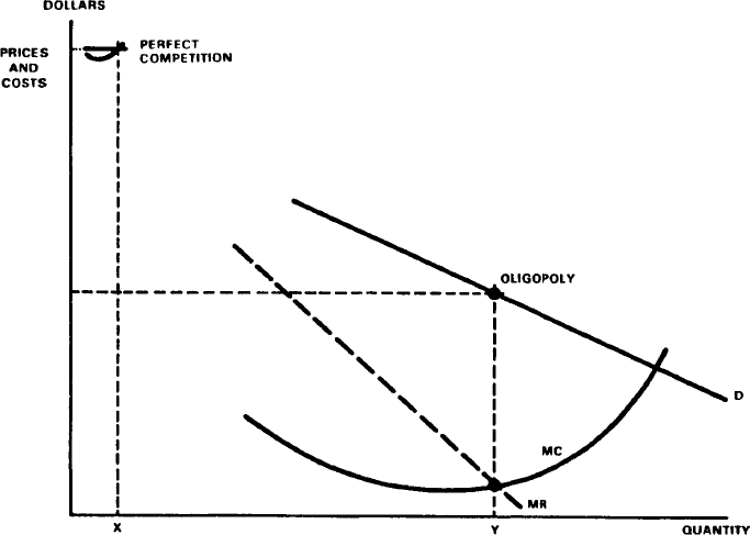
FIGURE 41:

OLIGOPOLIST PRODUCES MORE AT LOWER PRICE.

A Mixed Blessing for Firms

Now, how about the firm? How does competition benefit it? From the firm’s viewpoint, unlike that of the consumer’s, competition under a profit-and-loss system is not an unmixed blessing! Whereas consumers stand only to gain from competition that drives costs and prices down and increases quality of product, firms must either gain or lose as the result of competition.

As we saw in Chapter X, the free market puts constant pressure on the firm to cater successfully to the consumer as the only way to earn profits and avoid losses. Firms are able to retain their hold on consumers’ demand only via product differentiation or cost-and price-reductions. Failure to do so brings losses and possible banishment from the market. Furthermore, the more investors and stockholders prefer to invest in profitable firms (rather than in loss-ridden firms), the more will firms be under the gun to earn profits and avoid losses.

Competition Is War!

Ironically, the same free-market competition that is an unmixed blessing for the “sovereign” consumer can drive firms to run screaming for shelter. History reveals that every now and then some firms have sent up the cry, “Competition is war, and war is hell!” More than one firm has run to government to secure its protection from the fateful verdict of consumers’ dollar ballots and competition from rivals at home and abroad. Whether government protection takes the form of subsidy, bailout, tariff, price-fixing, so-called “regulation,” or guaranteed market, it can only serve to undermine the degree of consumers’ sovereignty in the market.4

The reason is that in a truly free market in which government refrains from tinkering with or hampering market competition, the only proper “protection” for the firm is to cater successfully to the consumer. The consumers’ dollar ballots are so powerful ultimately that we must alter our conception of market competition: that which superficially appears to be “rivalry” among firms is actually an indirect manifestation of the consumers’ fateful balloting. For example, if firm A outstrips firm B in the market place, and firm B closes down or shrinks in size, it is not firm A that is ultimately to blame for B’s fate. Blame must fall ultimately on the consumers who showed overwhelming preference for A over B. Thus, when firms cry “Competition is hell!” they are really paying indirect tribute to the fateful power of the consumers’ dollar ballots.

Summary

At the start, in Figure 33 we met the classic thesis that the PC firm outperforms the IC firm by producing more Q at a lower P than the bigger IC firm. We then explored the two paths that lead to this thesis; one path took us through the horizontal D schedule, the other went through the process of profit-maximizing by means of MC and MR. Things came to a head in Figure 38 which contains the curvilinear latticework that incriminates the IC firm merely because it has a sloping D schedule.

Finally, in denouement, we see that the case against the IC firm amounts to intellectual sleight-of-hand; after all, it is not the sloping D schedule that does in the IC firm so much as it is the oversight concerning the cost curves. However, none of this critique of the PC model should be construed as a whitewash of the big corporation. There is a case to be made against certain tendencies in corporate behavior, but it has little to do with atomism or sloping D schedules; it has more to do with business’ tendency to run to government for protection whenever the going gets rough in competition at home and abroad.

 

___________________

5A noteworthy analysis of the problem of defining competition is by P. J. McNulty, “Economic Theory and the Meanings of Competition,” Quarterly Journal of Economics (November, 1968).

6Important contributions to the understanding of open monopolies are by W. S. Leeman, “The Limitations of Local Price-Cutting as a Barrier to Entry,” Journal of Political Economy (August, 1956) and J. S. McGee, “Predatory Price Cutting,” Journal of Law and Economics (October, 1958).

7Joseph A. Schumpeter, Capitalism, Socialism, and Democracy (3rd ed., New York: Harper & Brothers, 1950), p. 86.

8There is historical evidence that business leaders in major industries, including the railroads, have sought federal protection against competition, at least since the 1880’s, via the Interstate Commerce Act and other so-called “regulation”. For example, see Gabriel Kolko’s two works. Railroads and Regulation, 1877-1916 (Princeton: Princeton university Press, 1965) and The Triumph of Conservatism (New York: The Free Press, 1963).

• 1See Thomas Sowell, Knowledge and Decisions (New York: Basic Books, Inc., 1980) for an elaborate analysis of how—despite the complex structures and environments of the modern division of labor—the free society and its market-price system generate, transmit, and apply “authentic” knowledge in the realms of economics, law, and politics. For an earlier treatment, see Friedrich A. Hayek, The Constitution of Liberty (Chicago: University of Chicago Press, 1960).
• 2Excellent examples of this type of supplementary work are John C. Goodman and Edwin G. Dolan, Economics of Public Policy: The Micro View (2nd ed., St. Paul: West Publishing Co., 1982), and Walter E. Williams, America: A Minority Viewpoint (Stanford: Hoover Institution Press, 1982).
• 3A notable exception is the above-mentioned text by Goodman and Dolan which analyzes public issues in terms of moral, political and economic criteria.
• 4For a philosophical treatment of morality in interpersonal relations, see John Hospers’ Human Conduct (2nd ed., New York: Harcourt Brace Jovanovich, Inc., 1982).
• 5Add to this the obfuscations, deliberate or inadvertent, of those messianic types who would deliver us from all our travails by imposing their illusions, myths and Utopian visions on the rest of us—and it follows that the task of discerning and explaining the true nature of economic existence becomes so much more difficult,
• 6For the rest, for the purpose of greater illustration and application of analysis to public issues and policies, I defer for the most part to the numerous useful works devoted especially to this purpose. These works, including books of readings, provide ample supplementary materials that illustrate at length how economic theory or principles manifest themselves in practice and how economic analysis can be applied to practical problems.
• 7Before proceeding to the chapter-by-chapter introductions, it is necessary to point out that economic tracts—mainly because of materialist bias—usually omit the very important moral dimension, a dimension that is nevertheless relevant to economic reality—to economics in practice. First of all, economics as a social science is fundamentally concerned with exchange—“interpersonal transactions.” Exchange is inherent in every production and trade activity. Thus, the market-price system may be regarded as comprising multitudinous exchange transactions. Since exchange also infuses every interpersonal transaction in society at large, it also constitutes the basic coordinating mechanism of that most complex network of interrelationships called “society.”
• 8Exchange transactions regarded as interpersonal activity necessarily involve the elementary moral question: by what moral principle should exchange between party A and party B be governed? Here only two basic principles are relevant: either the principle of nonviolence (non-aggression) or its opposite, violence (aggression). Violence and aggression can be identified simply by such acts as theft, killing and fraud.