Chapter VI. The Demand Side of the Market

CHAPTER VI THE DEMAND SIDE OF THE MARKET

The market place is a social-economic context in which suppliers and demanders face each other in repeated instances of exchange—actual and potential. The rates at which they exchange their goods and services and money constitute the “prices” of the market. As we shall see in Chapter VIII, it is the free and spontaneous interplay of demand and supply forces which determines the prices that tend to prevail in the market. Having already discussed the basic aspects of production and supply in Chapter IV, and the ramifications of wants in Chapter V, we now examine the demand side of the market in all of its relevance to the firm.

Demand vs. Wants

Our first task is to clarify the distinction between natural wants (i.e., desires, wishes, needs, appetites, etc.) and the concept of demand, a distinction already noted in Chapter II and Figure 5. When we talk about “wants” in economics, we have in mind the natural fact that all human action is broadly motivated by one or another desire, wish, or purpose. Furthermore, as we have seen, a want can be satisfied only by the application of means—time, effort, or wealth—that is, some expenditure, sacrifice, or cost. In other words, in a world of scarcity, wants by themselves do not help us very much; means must be acquired and applied to achieving the satisfaction of wants.

Here is where the concept of demand comes in: it encompasses not only the fact that a person has wants or goals, but that he also has the means to satisfy them effectively. Thus, in a barter economy, demand is exercised by means of producing and exchanging one’s own product for the products of other producers. By contrast, in the modern market economy, the means used for the purpose of exercising demand typically takes the form of money, which, as a means of payment, is exchanged for product. Besides money, other forms of wealth—such as financial assets—also serve as sources of purchasing power (albeit not as money proper), which must be converted into money before they can be accepted as a means of payment.

Demand vs. Needs, Consumption

Similarly, demand must be distinguished from the term needs, which we saw in Chapter V is a term used to emphasize a want to which one attaches a special degree of importance. “Needs,” like wants in general, are also handicapped by the fact that, by themselves, they do not possess the means to be satisfied; and just like wants, needs can only impel people to acquire means to satisfy them. Thus there is no “need” that can be satisfied without some effort or cost.

Before we proceed, we should note another important distinction of terminology—the difference between “demand” and consumption. Demand, as has been shown, is related only to the act of acquiring goods; in contrast, “consumption” represents that act of actually satisfying the want for which the goods were acquired. More precisely, demand is exercised by the use of means, through exchange or purchase transactions; however, the actual consumption of the goods thus acquired does not take place until the person actually uses them for the purpose of directly satisfying the given want or fulfilling the given goal.

More on Consumption

To be sure, a person’s ability to consume rests principally on one’s ability to exercise demand in the first place. Thus, demand is logically prior to consumption, and consumption is therefore predicated upon the exercise of demand. But this fact in itself does not imply anything as to when the final act of consumption will actually take place. For example, consumption may occur virtually simultaneously with the act of demand, as in the case of a frankfurter purchased at a hot-dog stand and eaten right there. Alternatively, consumption may occur only after a deferred period following the acquisition of the goods, as in the case of frankfurters purchased and stored in the refrigerator, pending a subsequent picnic or other occasion.

Furthermore, in economics, consumption has a much broader or general meaning than the narrow, materialistic meaning usually given to it by the layman. For example, economics classifies as consumers’ goods such things as leisure, music, spiritual worship and other intangible or non-material goods alongside such material goods as food, clothing, or jewelry—and for the same reason: any goods that have the capacity to directly or personally satisfy a want or purpose, be it material or non-material, must be classified as consumers’ goods. Hence, the act of personally using a consumers’ good is regarded as “consumption.”

Demand is Based on Production

As important as means are for the exercise of demand, equally important is the fact that, whether the economy is based on barter (direct) exchange or monetary (indirect) exchange, means must be acquired typically by productive effort. This productive activity yields purchasing power to the producer—whether in the form of (a) goods produced in the case of Robinson Crusoe and subsistence, direct-use economy, or (b) money income earned in the modern monetary economy. It is this productive effort which constitutes the basic sacrifice or cost involved in the acquisition, directly or indirectly, of the means to satisfy one’s wants. Since means are required to exercise demand in the market, and means must be acquired by productive effort, it follows that demand must ultimately be based on productive effort. Thus, demand is more than mere wants or needs.

All of this brings us to a fundamental implication. The fact that, on the one hand, wants cannot be satisfied without the use of means, plus the fact, on the other hand, that the means are scarce, imply the following: There is an inverse or opposite relationship between the quantity or extent of wants to be satisfied and the sacrifice or cost involved in achieving the satisfaction of wants. That is to say, the greater the sacrifice or the more it costs to satisfy a given want, the less of that want will a person seek to satisfy; conversely, the less it costs a person to satisfy the want, the more of it will he be induced to satisfy.

Demand vs. “Quantity Demanded”

Here we have the essence of the economic principle referred to as the law of demand. In order to see how economics formulates this law, we must first introduce and define the key, albeit simple, term quantity demanded, which is not to be confused with the term “demand.” Indeed, the term “demand” itself remains to be defined more precisely, since up to now we have used it superficially.

For convenience, the term “quantity demanded” will be expressed simply as “Qd.” Qd stands for the number of units of a good or commodity that a person would purchase at any given price. This term acknowledges the fact that, in the market place, goods of whatever class or grade are typically sold and purchased in units of numbers (e.g., one, two, or more), weight (e.g., ounces, pounds), or length (e.g., yard goods). Furthermore, prices in the market place are typically quoted in terms of such units; for example, the price of hamburger meat would be quoted at $1.50 per pound.

Since the term Qd includes the word “demanded,” it is evidently associated with the act of acquisition (via purchase or exchange) and not with the act of consumption. As a rule, therefore, Qd refers to the rate of purchase—that is, the number of units that a person would purchase at a given price—and not to the rate of consumption. Thus, to paraphrase the implication stated at the end of the previous section, economics asserts: there is an inverse or opposite relationship between the price of a given good and the Qd of that good. Specifically, the higher the price asked for a unit of a given good, the smaller will be the Qd; the lower the price, the greater will be the Qd. This proposition brings us pretty much to the heart of the law of demand.

Determinants of the Quantity Demanded

In order to fully appreciate the law of demand, one more important bridge remains to be crossed. The reason is that while the law of demand assumes that price is the only determinant of the Qd of a product, in reality this is not strictly true. As we shall now see, there are several other determinants of Qd—other than price, hereinafter referred to as non-price determinants, for convenience—that also exert important influence on the Qd of a given product. So, let us first examine each one of these non-price determinants, and thereby gain a better perspective on the law of demand.

What else does the Qd of a product depend on, other than the price of the product itself? We have already seen that the price of the product would be a “negative” or inverse influence on the Qd: a lower price would induce an increase in Qd, whereas a higher price would cause a decrease in Qd. . . . However, to be more precise, we should add an important proviso: provided that other (non-price) determinants of Qd are assumed to be passive and uninfluential. Why is this proviso necessary? Because these other, non-price determinants can influence Qd even when the price of the product has not been changed by the firm; that is, changes in one or more of the non-price elements could cause Qd to change even when the price of the product itself remains unchanged. The following examples help us to understand this.

Income and Population

The first non-price determinant of Qd that comes to mind is a fairly obvious one: the consumer’s income or other purchasing power or wealth. Thus it would follow that, other things being equal, the greater a person’s purchasing power, the greater would be his Qd of a given product. In other words, the rate at which we buy things depends on how “rich” we are. A person’s purchasing power depends primarily on his income as well as on accumulated savings from past income; the latter may take the form of financial investments or assets (e.g., securities, deposits) that are readily convertible into money (i.e., are “liquid”).

Another important determinant of Qd, also fairly obvious, is the size of the household unit, or of the total population. Other things being equal, we would expect that the greater the number of people in the household, or in the population as a whole, the greater would be the Qd of the given product, and vice versa.

Subjective Value: Tastes or Preferences

Another important determinant of Qd is something we discussed at length in Chapter V: subjective value, or the degree of importance attached to a unit of a given product. Thus, other things being equal, the greater the subjective value, the higher the price one would be willing to pay; conversely, the less important the product, the lower the price one would be willing to pay. If we recall, subjective value depends on two things: the character of taste, or the preference-scale ranking attached to the product; and the amount of stock of the given product already possessed by the consumer (the law of marginal utility). Thus, with reference to the preference-scale, the higher the rank of the product on a person’s preference-scale, the higher the price one would be willing to pay; conversely, the lower the rank held by the product, the lower must the seller’s price be in order to induce a purchase.

A few examples will suffice to illustrate this aspect of subjective value. Advertising by firms, one of the most familiar institutions in the market place, serves two important functions: the one is to inform consumers about the product—its price, quality, location of sellers, etc.; the other is to persuade consumers that they cannot live without the given product, hoping that the consumer will then place the given product on a higher rank of his preference-scale. Medical reports on the link between tobacco smoking and lung cancer have caused cigarettes to drop to a lower rank or disappear altogether from many people’s preferences. Studies on the relationship between diet and health have played havoc with the position of eggs, butter, and processed foods in our preferences. Finally, changes in fashion play similar havoc with the position of older models or styles in cars and clothing, as well as living patterns in general.

The Law of Marginal Utility

Similar effects on subjective value can be exerted by variations in the amount of stock already possessed by the consumer of a given product. This is the aspect of subjective value where the law of marginal utility becomes relevant. If we recall, the law asserts the following: the smaller the stock, the higher is the marginal utility (MU) or subjective value attached to a unit of the product; conversely, the larger the stock on hand, the lower is the MU attached to each unit.

Now, applying this law to prices, we come up with the following: the smaller the quantity supplied by sellers and the higher the MU therefore attached by the consumer to each of the fewer units, the higher is the price that the consumer is willing to pay for any unit of the product; conversely, the greater the quantity supplied by sellers and the lower the MU therefore attached by the consumer to each unit of the available supply, the lower must the price asked by the seller be in order to induce consumers to buy more units.

A clear example of the relevance of the law of MU was the gasoline shortage in late 1973. At the time of the oil embargo, in the fall of 1973, the supply of refined gasoline reaching the market had dropped significantly. When car drivers realized that considerably less gasoline would be available, it did not take long for them to adjust and begin to attach a higher MU to each gallon of gas obtained after much search and waiting in line at the gas pump. Simultaneously, they also adjusted upward the price they were willing to pay for each of the more precious gallons.

Complementary Products

Another important set of influences on the Qd of a given product involves the effect of changes in the price of other related products. Many products are “related” to each other in one of two possible ways—as complementary products or as substitute products. Complementary products typically go together; that is, they are usually jointly consumed. Good examples are bread and butter, beer and pretzels, cars and gasoline. As a consequence, a change in the price of one of the pair would be expected to exert an opposite effect on the Qd of the other. For example, a rise in the price of gasoline would be expected to cause a drop in car-driving—more precisely, a drop in the Qd of transportation mileage by automobile; conversely, a drop in the price of gasoline would be expected to induce an increase in car-driving—that is, an increase in the Qd of transportation by automobile.

Substitute vs. Complementary Products

Similar considerations apply to substitute products, that is, products that are regarded as “rivals” or “competitors” to each other with respect to a given use or purpose. Good examples are butter and margarine (for cooking); paper and cellophane (for wrapping); natural fibers like silk, cotton, and wool as against nylon, dacron, orlon, and other synthetic fibers (for clothing and textiles). Since these commodities are substitutable for each other in specific applications, it stands to reason that a rise in the price of the one (say, butter) relative to the price of the other (i.e., margarine) would induce a rise in the Qd for margarine, as people are induced to shift from butter to margarine. Conversely, a drop in the price of butter would be expected to induce a drop in the Qd for margarine, as people are induced to shift from margarine to butter.

In the case of complementary products, price changes in one of the pair are expected to induce opposite changes in the Qd of the other complementary product. Thus, a rise in the price of gasoline is expected to induce a drop in the Qd for transportation by car. On the other hand, in the case of substitute or rival products, price changes in the one are expected to induce Qd changes in its rival products in the same direction. Thus, a rise in the price of paper relative to its rivals (say, cellophane wrap) is expected to induce a rise in the Qd for cellophane. In general, therefore, changes in the price of one of the “related” products would be expected to induce Qd changes in the other of the related products.

Before proceeding, we should note that the preceding, non-price determinants of the Qd—such as income, subjective tastes or valuations, and size of households—were truly “non-price” in character. However, in the present case we were dealing with the possible effects of price changes in related products, so that, strictly speaking, the subject is not “non-price.” For convenience, however, the effects of price changes in related products are treated as a “non-price” determinant.

Expectations of Future Price Change

A final, but nevertheless important set of determinants involves expectations about the future. This dimension of influence is made relevant by the fact that, so long as such determinants of Qd as price and income are subject to change, the future becomes uncertain. That is to say, tomorrow’s price will not necessarily be the same as today’s price, since it may be higher or lower than today’s price; nor will tomorrow’s personal income necessarily remain the same as today’s. As a consequence, today’s Qd will depend not only on today’s price and income, but also on tomorrow’s price and income.

For example, assume a situation in which prices have been falling, as during periods of price “deflation.” A consumer therefore has grounds to expect that tomorrow’s price (say, of clothing) may be still lower than today’s price. Given such expectations it would be reasonable for the consumer to postpone his planned purchase of clothing until tomorrow, since he would prefer to buy at tomorrow’s expected lower price rather than at today’s relatively higher price. Conversely, assume that prices have been rising, as during periods of price “inflation.” The consumer would therefore reasonably expect that tomorrow’s price could be higher than today’s price, and consequently decide to hasten his purchase and buy today rather than delay his purchase until tomorrow, since today’s price appears relatively lower compared to tomorrow’s expected higher price.

In sum, therefore, expectations of a change in tomorrow’s price compared to today’s price would reasonably influence the consumer’s rate of purchase (Qd) today: an expected higher price would induce a hastening in the rate of purchase (i.e., an increase in the Qd today), whereas an expected lower price would induce a postponement of purchases (i.e., a decrease in today’s Qd). So long as prices are not stable or constant, but are either rising or falling, it is clear that tomorrow’s price will not be the same as today’s. Therefore, at any given time, the consumer is faced with not one price but two prices: today’s price and tomorrow’s possible price. As a consequence, he is prompted to decide which of the two prices will be the relatively lower, and decide his Qd accordingly, that is, at the relatively lower price, according to the law of demand.

Expectations of Future Income Changes

Similar considerations apply to expectations of change in one’s future income. For example, an expected increase in salary or wages due to an expected promotion would obviously herald an increase in future income; conversely, an expected reduction in working hours or loss of one’s job, due to a slackening of business, would lead one to expect a drop in tomorrow’s income. In either case, the expected change in tomorrow’s income would induce a reasonable adjustment in today’s rate of purchase (Qd).

For example, if a worker expects to receive a wage increase in the nearby future, it would not be unreasonable for him to spend that money now, in anticipation of his increased future income and on the assumption that “the money is as good as in the bank,” so to speak. Similarly, if Congress announced a cut in tax rates effective within a few months, it would not be unreasonable for taxpayers to spend that money now. (Economists attribute the stepped-up rate of spending in the latter half of 1963 to the anticipated Kennedy tax-cut scheduled for 1964.) In both cases, the effect of the anticipated increase in future income is an inducement to increase the current rate of spending (Qd). The opposite would happen in the case of anticipated decreases in income. That is, wage-earners would be expected to reduce their current Qd if faced with layoffs or curtailed working hours; taxpayers, too, would be expected to spend less today if faced with a tax increase tomorrow.

What About Changes in Supply?

Have we left anything out? Well, what about the supply of the product—that is, couldn’t changes in supply conditions cause changes in Qd? For instance, couldn’t increased supply cause an increase in Qd, and vice versa? Economics would answer as follows: changes in supply can affect Qd only indirectly, through the prior effects on the price of the product. Thus, other things being equal, an increase in supply would first have to cause a drop in price before it could induce a larger Qd; conversely, a decrease in supply would first have to cause a rise in price before it could induce a smaller Qd.

Restatement of the Law of Demand

Thus, we see that the quantity demanded (Qd) of a product in the present can be influenced not only by the price of the given product but also by a variety of non-price determinants. As a consequence, it would be reasonable to conclude that, even if the current price of a product remained unchanged, the current Qd could nevertheless be induced to change due to a change in one or more of the non-price determinants. In any event, the firm faces a difficult task in assessing which of the several non-price determinants is influencing the Qd for its product and to what degree. It is one of the primary functions of market research to study the importance of each of these determinants of market demand.

All of this enables us to state the law of demand with greater precision than before. First comes the general statement of the law of demand: there is an inverse, opposite, or negative relationship between the current price of a good and the quantity demanded (Qd) of this good, provided other things (i.e., the non-price determinants) remain the same. From this general principle are derived the two important corollaries: (1) other things remaining the same, at a sufficiently higher price the Qd will be expected to decrease; (2) other things remaining the same, at a sufficiently lower price the Qd will be expected to increase.

Before we proceed, it is important to note that the law of demand applies only to the case where the price of the given product is changed relatively to, or comparatively to, the prices of other products. Thus, a decrease in the price of product X can be regarded as a “lower” price only when compared to what happens to other product prices, especially substitute or similar products. Thus, a decrease in the price of product X can be regarded as a “lower” price only when compared to what happens to other product prices, especially substitute or similar products. If prices of other similar products are decreased in the same proportion as product X, then the drop in X’s price is not a comparatively lower price. The price of X is truly “lower” only when it is decreased while other prices remain the same, or decrease less than X’s price, or even increase. Conversely, X’s price cannot be regarded as a “higher” price unless it is increased more than in proportion to the prices of other similar products, that is, only if other prices do not increase, or increase less than X’s, or even drop.

The “Ceteris Paribus” Proviso

We can now see more clearly why the law of demand is based on the special assumption that “other things remain the same,” and that the price of the given product is the only determinant of its Qd. The proviso “other things remaining the same” has become known in its latin form as the ceteris paribus clause (which literally means: other things being equal). In the real world, of course, it is more reasonable to assume that the non-price or “ceteris” determinants do not remain fixed or unchanged, and that any given change in Qd could be a result of a non-price change as well as of a price change by the firm. However, for the purpose of economic analysis, which seeks to intellectually isolate the effect on Qd of the price alone, it is logically necessary to abstract from the non-price determinants and assume that they are, for the moment, passive or dormant.

In other words, the law of demand assumes that at any given moment it is reasonable to assert that the Qd of a given product X is influenced only by the price of X—that is, market exchange involves only P’s and Q’s, so to speak. This special assumption of ceteris paribus is a kind of “mental experiment.” It is the closest that economic analysis comes to duplicating a controlled laboratory experiment, as in the physical sciences, where it is possible to isolate and exclude all variables or determinants except one. In the human sciences, including economics, it is impossible to conduct such physically controlled experiments; the only intellectual recourse left, then, is the method of “partial analysis,” which uses the logical device of the ceteris paribus proviso.

Law of Demand Is Not “Automatic”

One additional explanation is needed. We have deliberately used the word “sufficiently” in the phrases “at a sufficiently higher price” (corollary 1) and “at a sufficiently lower price” (corollary 2). This is to exclude the case of very small or minute changes in price which, in practice, may not induce any significant change in Qd. Realistically, it would not be reasonable to expect that just any size of price increase (or decrease) would necessarily induce a decrease (or increase) in Qd; indeed, it is very possible that a very small or insignificant change in price would have practically no impact on Qd.

For example, it is possible that during the early stages of the gasoline shortage in the fall and winter of 1973-74, the relatively small initial increases in gasoline price did not in themselves cause any significant drop in Qd of gasoline. However, such unresponsive changes in Qd to the rise in prices would not constitute a contradiction of the law of demand, since, properly stated, the law pertains only to relatively significant of “sufficiently” large changes in price. Thus, whereas a rise in gasoline price from, say, 40 cents to 50 cents a gallon might not in itself cause any significant drop in Qd, a “sufficiently” great increase from 40 cents to 80 cents, say, could be expected to cause a significant drop in Qd.

In other words, the law of demand does not assume that people react automatically or mechanically (i.e., immediately) in response to just any size of stimulus (e.g., a price increase). Indeed, it is rather usual for people not to react significantly to small or tiny stimuli, and it is only when stimuli are “sufficiently” large that they will react and adjust in reasonable ways.

Furthermore, even when the stimulus is substantial, people will respond only after they are able to discover the best way of adjusting to the stimulus—all of which will take some time. In the case of a price stimulus—for example, an increase in price—it will take some time at least before the consumer can adjust (a) by switching to a substitute product, or (b) by deciding to do with less of the given product, which involves a distinct change in taste or preference.

Graphic Presentation of Law of Demand

We are now at the point where the law of demand can be illustrated graphically. The graph shown in Figure 8 is based on the fact that the law of demand involves only “P’s and Q’s,” that is, prices and quantity demanded; hence, only a two-dimensional graph is required. The vertical scale or “axis” on the left represents the various prices that could be charged per gallon of gasoline, rising up from lower to higher prices. The horizontal axis represents the quantities that would be demanded at various prices, showing increased quantities as you move from left to right.

Of course, Figure 8 is not based on actual market data, which could be obtained only by a market research survey. It is merely an illustration of what an economist might expect to find if he undertook a market survey by asking car drivers the simple question: “How many gallons of gasoline would you purchase at various prices, say, from 30 cents up to $1.20?” The resulting sample data represent aggregation of the data gleaned from the survey responses.

Each dot in the graph represents two bits of information: a given, potential price that could prevail in the market, and the corresponding number of gallons that would be demanded by each car driver. That is, each dot represents a given “P and Q,” so to speak: a given price (P) and the corresponding quantity demanded (Qd). Thus, at $1.20 a gallon, very few gallons would be demanded, but, at successively lower prices, more and more gasoline would be purchased.

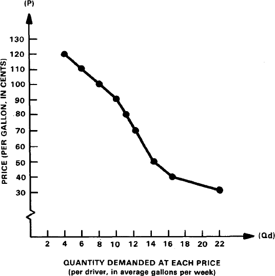
FIGURE 8:

DEMAND FOR GASOLINE BY PASSENGER CAR DRIVERS.

The Demand “Schedule”

Notice that the dots are linked to each other in sequence by straight lines, and form what is known as the demand curve. Ideally, the demand curve would be derived from data collected by a market survey, with the series of dots representing a discrete array of pairs of prices and Qd’s. Indeed, the original statistical data obtained in such market surveys might very well assume the tabular form presented below in Table I. Notice therein the inverse relation between the prices and Qd’s, with the P’s going from high to low while the corresponding Qd’s go from low to high. Together, this array of pairs of P’s and Qd’s, presented in tabular form, constitutes the demand schedule.

Table I

DEMAND FOR GASOLINE BY PASSENGER-CAR DRIVERS

(in gallons)

Price (per gallon)	Weekly Quantity Demanded (per driver)
$1.20	4
1.10	6
1.00	8
.90	10
.80	11
.70	12
.60	13
.50	14
.40	16
.30	22

An “Instantaneous Snapshot”

Thus, Figure 8 is an illustration of the law of demand by means of the demand curve. Here the Qd’s are shown to vary only in response to the different possible prices—on the ceteris paribus assumption, of course, that personal tastes, incomes, and other non-price determinants of Qd are dormant. In this sense, therefore, the curve gives us, in effect, an instantaneous snapshot of how people “feel” about gasoline prices when expressed in terms of gallons demanded. It is this overall view of the various possible pairs of P’s and Qd’s which is designated as the total “demand” schedule, in contradistinction to the specific “quantity demanded” which is related to a given price.

Thus, even if we had no precise idea of the specific magnitudes that the market survey would reveal, the law of demand would lead us to expect that the demand curve would have this overall characteristic slope: downward from left to right. So, assuming the present price was 50 cents a gallon, a price increase to 60 cents a gallon would be expected to cause a drop in Qd to 13 gallons a week, whereas a price decrease to 40 cents would be expected to induce an increase in Qd to 16 gallons.

The “Elasticity” of Demand

In this connection it should be noted that, while all demand curves possess the characteristically general slope downward (from left to right), not every demand curve necessarily has the same degree of slope, technically referred to as elasticity of demand. The following Figure 9 illustrates three different schedules, each having a different degree of slope or elasticity. Curve D1 on the left would be classified as “inelastic,” curve D2 in the middle displays “unitary” elasticity, while curve D3 on the right would be regarded as “elastic.” Notice that the “curves” have been drawn, for convenience, as straight lines in order to emphasize the general degree of slope of the entire schedule. A more detailed analysis of demand elasticity, and the critical importance of the concept, will be the subject of the next chapter.

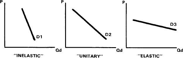
FIGURE 9:

DIFFERENT DEGREES OF ELASTICITY OF DEMAND

As a final note, it should be stressed that the demand schedule does not constitute an actual rate of purchase, but merely an indication of people’s readiness to buy, based on their wants and modified by their economic ability, that is, their purchasing power. In other words, the use herein of the term demand, by itself, will connote not a sense of actuality but rather of potentiality.

“Shifts” of the Demand Schedule

We come now to an important question: What happens to the demand schedule when the basic ceteris paribus assumption of the law of demand—that non-price determinants are dormant or unchanging—is relaxed, and these determinants are allowed to change, as they do in the normal course of events? That is to say, what is the effect on demand of a change in one or more of the non-price determinants? For example, what happens to the demand for product X when people’s incomes or tastes and preferences change? Well, it all depends on whether these determinants increase or decrease.

For example, if there is a general increase in income in the community—of wages, say—then we could expect that people would be able to purchase more units at each possible price. This can be seen in Table II, where the quantity of gallons that would be purchased at each possible price (from $1.20 down to 30 cents) would be expected to increase in varying degree as shown for Period 2. Graphically, the resulting change in the state of demand is shown in part A of Figure 10. That is to say, the entire schedule or curve of D would be expected to shift from position D1 to D2, from left to right, indicating that, at all possible prices, people would be willing and able to buy more. A similar graphic effect would be expected if, instead of an income increase, there occurred an increased taste or preference for a given product.

The same reasoning applies to the case of a decrease in incomes in the community. Here we would expect that people, with reduced purchasing power, would be induced to buy less at each possible price, and the demand schedule would correspondingly undergo a “shift” to left, as in part B of Figure 10.

Table II

AN INCREASE IN DEMAND FOR GASOLINE BY PASSENGER-CAR DRIVERS

Price (per gallon)	Weekly Quantity Demanded (per driver)
Price (per gallon)	Period 1	Period 2
$1.20	4	5
1.10	6	7
1.00	8	9
.90	10	11
.80	11	12
.70	12	13
.60	13	14
.50	14	15
.40	16	19
.30	22	27

Some Comments on Demand Shifts

It should be noted that in all such instances of change in non-price determinants—and in the corresponding shifts of demand curves—it is not possible to predict exactly the extent or degree of change; only the general direction of shift is predictable.

Finally, it should be stressed that a shift in the entire demand schedule cannot be caused by a price change—only by a non-price change. True, laymen customarily say such things as, “rising prices cause a drop in demand,” or “falling prices cause an increase in demand.” For economics, this language is not sufficiently precise: in each statement the underlined word “demand” should be replaced by “quantity demanded” to make the statement correct. Price changes can only cause specific changes in Qd along a given unchanged demand schedule (“a movement along the curve,” so to speak); on the other hand, only non-price changes can induce “shifts” of entire demand schedules.

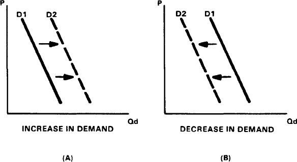
FIGURE 10:

“SHIFTS” IN THE DEMAND SCHEDULE.

The Role of Market Research

How would the firm become aware of such a shift in demand? First of all, we must be sure that the change in Qd’s was not caused by a change in price by the firm; that is, the selling prices of firms must be assumed to have remained unchanged, so that any change in Qd cannot be attributed to a price change but rather to a change in one of the non-price elements. Thus, if a firm has not changed its price, and yet the Qd for its product has either increased or decreased, then it is certain that one or more of the non-price determinants were at work.

This raises the question: How can the firm discover which one or more of the non-price determinants of demand is at work, and to what extent? In this connection, market research projects become very relevant. The firm may have to undertake market research studies on each of the possible non-price determinants. Such studies, even though very costly, may be worthwhile if the firm believes that knowledge of demand determinants would improve its ability to plan future production and marketing, and leave it better off than otherwise.

Explaining the Law of Demand

We have now reached a crucial point in the analysis. So far we have presented mainly a description of the law of demand, without really giving the rationale behind it, and without explaining why we would expect the demand curve to slope generally the way it does. Although the law of demand makes a lot of common sense, it is nevertheless important to explain precisely why this is so. Some writers have attempted to explain the “why” of the demand curve, and it is useful to briefly examine their efforts.

Substitution Effects

One explanation of the law of demand is based on the notion of the substitution effect, which assumes that all products have “substitutes,” either in the form of rival brands or rival products, as in the case of butter vs. margarine. Thus, when the price of a given product X is decreased, potential buyers are supposed to be induced to switch their buying from other products to product X, and thereby cause an increase in the Qd of X. However, the trouble with this theory is that it does not necessarily follow.

This can be seen in the case of a price decrease. For one thing, there is no certainty that product X has any substitutes at all from which loyalty can be switched to it. Nor is it necessary that the savings resulting from the lower price of X will inevitably be used to buy more of X itself rather than more of some other unrelated product.

What about an increase in the price of product X? The substitution effect would be expected to work as follows: a higher price for X would induce purchasers of it to buy less of it, and thereby cause a decrease in Qd of X. Thus far, then, the “substitution” theory is still consistent with the law of demand. Beyond this, however, it falls down: substitution effects do not necessarily follow.

First of all, unless we know something about the price-elasticity of demand for X (to be discussed in Chapter VII), it is not even certain that a reduced Qd will yield any savings at all. Indeed, in the case where few or no substitutes are available, it is possible to get the curious result that the smaller Qd is associated with an increase in total expenditures on X (as would be expected in a product like gasoline, which people cannot easily cut back if they are heavily dependent on automotive transportation). Hence, if there are no savings to start with, there can be no increment of money, at least in the short run, with which to do any switching to substitutes.

To be sure, if substitutes are sufficiently available, the substitution effects could easily occur, as the higher price of X induces people to switch to the substitute brand or product and causes a decrease in the Qd of X. Furthermore, if product X is of the type that simply does not command any strong preference or attachment among its customers, and people find they can easily do without it, (i.e., the demand for it is very “elastic”), then its Qd could be expected to decrease as a result of its higher price; however, in this case there need not ensue any substitution effects.

Income Effects

Thus, the substitution effect is not a sufficient explanation of the law of demand. Another explanation offered by some writers is based on the notion of the income effect, which correctly assumes that changes in the price of products affect the purchasing power of one’s income. That is to say, a lower price for product X makes buyers of X “feel richer,” whereas an increase in price makes them “feel poorer.” However, this does not necessarily follow.

Let us first take the case of a decrease in the price of X. The fact that the lower price yields a kind of savings to buyers of X does not necessarily imply that this increment will be devoted to increased Qd of X itself. Indeed, it could just as well be devoted to some other unrelated products. But, for argument’s sake, let us suppose the savings are used for buying more of X: unless we know something about the price-elasticity of demand for X (to be analyzed in Chapter VII), it is possible to come upon the curious result seen in Table I: for example, the drop in price from 40 cents to 30 cents could be associated with an increase in total expenditures—from $6.40 (40 cents x 16 gallons) to $6.60 (30 cents x 22 gallons)—that is, an increase in total spending of 20 cents that could be attributed as much to a strong subjective preference for additional travel as to any income effect per se.

How would the income effect occur in the opposite case of a price increase? The assumption is that, at the higher price, the decrease in Qd is induced by the feeling of being made “poorer” by the price raise. However, here too it is not entirely true that the reduced Qd is induced only by the impoverishment effect. Again, in Table I, we see a case where a price raise, say from 40 cents to 50 cents, would be associated with an increase in total expenditures—from $6.40 (40 cents x 16 gallons) to $7.00 (50 cents x 14 gallons). That is to say, even though the price raise caused a drop in Qd, the fact is that total spending increased by 60 cents, revealing not an income effect but rather a lingering strong preference for car driving, such that drivers are willing to pay more money (in total) for fewer gallons of gasoline.

People Prefer Lower Prices

In summary, then, neither the substitution effect nor the income effect is sufficient to explain why the demand curve slopes the way it does. In this connection, it should be noted, there is a third type of explanation: the idea that the law of demand is merely a description of how demanders in general and consumers in particular “feel” about prices. Thus there follows this proposition: people prefer lower prices to higher prices. That is to say, in terms of the law of demand, this can be expressed as follows: preference for lower prices is reflected in the greater quantities demanded, whereas rejection of higher prices is reflected in the fewer units purchased. This proposition, that people prefer lower prices, turns out to be, in effect, a reverse way of expressing the law of demand: for any given quantity to be purchased, a person would prefer to buy it at a lower price rather than at a higher price; indeed, the lower the price, the better.

The Least-Cost Principle

Let us pursue this line a bit. The money price asked by the seller of a good in the market place represents a kind of cost or sacrifice that the demander must make in order to acquire the good. The element of sacrifice lies in the fact that the demander must give up leisure and go to work in order to earn the money with which to pay for the desired good. We can now restate the preceding proposition: for any given want or goal, the lower the cost or sacrifice involved, the better—other things being equal. Logically, this leads us to conclude that the least cost or sacrifice is the best.

Indeed, this leads us to yet another proposition: in order to achieve any given purpose or goal, man prefers the least-cost method, other things being equal. This would be thoroughly consistent with the maximizing principle (see Chapter V). As we recall, the maximizing principle asserted that man chooses to do that which he expects will leave him better off than otherwise. Since, in our present case, lower money prices, lower costs, or lesser sacrifices clearly leave man better off than otherwise, it is reasonable to assert that man would prefer not only the lesser cost (to the higher cost) but, indeed, the least cost.

When all is said and done, however, the fact remains that the least-cost principle is merely consistent with the law of demand (and the maximizing principle), but cannot serve as a sufficient explanation of why the demand schedule slopes downward from left to right. The reason is that it, too, can be criticized on the same ground as the income-effect explanation. The income effect operates on the premise that lower prices make us feel “richer;” the least-cost principle is relevant primarily to the case of a price decrease. In either case, the increased purchasing-power effect caused by a price reduction does not necessarily imply an increase in Qd of product X itself: the “income” increment could just as well be devoted to other, non-X products.

Again, The Law of Marginal Utility

This writer believes that the best all-around explanation of the law of demand is the law of marginal utility (Chapter V). The best way to see this is to raise the question: For whom does the law of demand have the greatest practical significance? Clearly, for the firm or the seller in general. As a first approximation, what the law of demand says to the seller is simply this: if you want to sell more (i.e., induce a greater Qd), you will have to reduce your price sufficiently; conversely, if you want to withhold supply from the market and offer fewer units for sale, then you can raise your price and this will reduce the Qd. But this still is begging the question; we have to invoke the law of MU, especially its corollaries.

First let us apply the law of MU to the case of a price reduction. Relevant here is the corollary on diminishing MU, which asserts that, other things being equal, an increased stock of a given good X is associated with a diminished subjective value attached to any one unit. How does this tie in with the law of demand? In this way: if the seller wants to sell more units of a given good X to people for whom each unit of this good is subject to a diminishing subjective value (i.e., because more units are available), then the seller must reduce his per-unit price sufficiently in order to induce people to buy more.

In other words, the buyer could not be expected to be willing to pay the same price for additional units of good X since, for him, acquisition of additional units is subject to the law of diminishing MU. Only a lower price per unit will induce him to buy more units. A very familiar example is the “economy-size” approach used in retail selling of detergents, coffee, and other consumers’ goods: compared to the smaller-size package, the larger (economy) size package is priced so that each ounce or pound of the good costs less than in the smaller package.

Similar reasoning applies to the case of a price increase. Relevant here is the corollary on increasing MU, which asserts that, other things being equal, a decreased stock of a given good X is associated with an increased subjective value attached to each unit. This ties in with the law of demand as follows: if the seller makes fewer units available for sale to buyers, for whom each unit of this good would be subject to an increasing subjective value (i.e., because fewer units are available), then the seller could raise his price and expect to get it.

In other words, people would be willing to pay a higher price for each unit, albeit in fewer units than before, since each unit is now subject to the law of increasing MU. Here, too, the economy-size approach is relevant, although in reverse: compared to the larger-size package, each unit (e.g., ounce) of the smaller-size package is priced higher than in the larger package.

Are There Exceptions to Law of Demand?

One problem remains: people sometimes object that the law of demand does not apply as a general rule—indeed, they claim there are exceptions to the law of demand which destroy its general validity. We shall examine a few of these alleged “exceptions” and see why they fail to prove their case against the law of demand.

Before we proceed, however, we should remember that the law of demand is concerned only with the relation between prices and quantities demanded (Qd’s). It follows therefore that each alleged exception to the law of demand—in order to prove its case—must be framed strictly in terms of this exclusive relationship between prices and Qd’s, albeit in the opposite sense; that is, an alleged exception must be able to show that (a) a lower price will induce a decrease in Qd, or (b) a higher price will induce an increase in Qd.

Selling More at Higher Prices

Let us first take up a familiar general case: The drug store which, after noticing that its bottles of aspirin did not sell very well at the discount price of 19 cents for 100 tablets, decided to raise the price to 49 cents! To its pleasant surprise, the aspirin sold much better at the higher price. This example is often given as an illustration of how a lower price induced people to buy less of the product, not more, thus contradicting the law of demand.

Is this really an exception to the law of demand? The first thing to notice is that: Was it only the lower price that had first induced a smaller Qd? Was it only the higher price that induced the increased Qd? It is well to recall that an exceedingly low price—such as the 19-cent price—may connote a product of lower quality as well, such that the lower price might induce a decrease rather than an increase in Qd! In the same vein, it is also well-known that a higher price for a given product often connotes to people a product of higher quality as well, such that the higher price could, not surprisingly, induce a greater desire to buy and an increase in Qd. Both of these cases appear to be clear contradictions of the law of demand.

Aspirins Fail the Test

To return to our aspirin case, it is relevant to ask again: Was it the lower 19-cent price itself that deterred purchases, or was it rather the fact that the low price also connoted inferior quality, therefore making the product not worth buying at all? Conversely, was it the higher 49-cent price itself that induced increased Qd, or was it rather the fact that the higher price connoted superior quality and therefore made the product more attractive?

To put this another way, in order to make the aspirin example a proper test case of the law of demand the following procedure would have to occur: at the same time that the seller raises his aspirin price from 19 cents to 49 cents he informs the customer that the 49-cent price is for the very same bottle that he could still buy at 19 cents—and then asks the customer: “Do you prefer to pay the 49-cent price or the 19-cent price for the identical commodity?” The outcome is predictable: For any given product, people would prefer to pay lower prices to higher prices, and the law of demand would still prevail.

In fact, of course, the drug store did not do this, and consumers were unaware that the aspirin quality was the same even at the higher price. Indeed, it was this ignorance of quality which explains why the Qd was greater at the higher price than at the lower price. Furthermore, the persistent tendency of sellers to resort to “sales” and “slashed prices,” in order to sell out goods at a faster rate than at the former higher prices, is testimony to our contention that the law of demand remains intact.

Prestige Goods

Another alleged exception to the law of demand involves the class of products known as prestige goods. Familiar examples include mink coats and Rolls Royce cars, whose prices are characteristically very high. The allegation claims that it is the higher price of these goods that induces a greater Qd than otherwise. In rebuttal, however, it is not the higher price itself that induces the greater Qd, but rather the status or prestige attached to the higher quality of the product. That is, people are willing to pay a higher price for the added prestige or status.

Furthermore, the fact that a mink coat, for example, is of a higher quality than, say, a silver fox coat, means that it must be classified as a different type or grade of product, and therefore does not belong on the same demand curve as silver foxes or other lower-grade furs. That is, a separate demand schedule must be drawn for each different type or grade of product. Thus, the demand schedule for a given grade of mink coat would be expected to reveal the familiar downward slope, left to right, associated with the law of demand; in this case, people would certainly not pay a higher price if they knew they could get the very same coat at a lower price.

Price Expectations

A final set of alleged exceptions involves price expectations. Let us first take the case of expectations of rising prices, as during a period of price inflation. As we saw above, expectations of higher prices tomorrow would be expected to induce a greater Qd today. Hence, it is alleged that this is an example of how higher prices can induce a greater Qd, thereby contradicting the law of demand. Actually, this allegation involves a distortion: it is not tomorrow’s higher prices that induce the greater Qd, but rather the realization that today’s prices are relatively lower than tomorrow’s expected higher prices; it is this realization that induces us to buy more today than usual. Hence, the law of demand remains intact.

The opposite case involves expectations of falling prices, as during a depression period marked by price deflation. As we saw above, expectations of lower prices tomorrow would be expected to induce a smaller Qd today. Again, the allegation claims that this contradicts the law of demand, since it shows that lower prices cause a drop in Qd and not an increase. This, too, is a distortion: it is not tomorrow’s lower prices that reduce today’s rate of purchase, but rather the realization that today’s prices are relatively higher than tomorrow’s lower prices. That is, at today’s relatively higher prices it pays to postpone purchases until tomorrow, when prices will actually be lower. Once again, the law of demand comes through unscathed.

Conclusion

A careful review of the alleged exceptions to the law of demand reveals a common characteristic: each basically involves a non-price determinant of Qd. This includes the case of price expectations, which we have classified among the “non-price” determinants. Since the law of demand involves only the relation between prices and Qd, it cannot be contradicted by cases that hinge on non-price determinants.

Foundations of the Market Price System