Foundations of the Market Price System

CHAPTER VIII HOW THE MARKET DETERMINES PRICES

Prices, prices everywhere—indeed, prices are the most widespread aspect of the market place. And the market place is the preeminent theater of exchange transactions in our lives—the stage upon which we offer each other the services of our labor power, savings, or other wealth, in order to earn the income with which to buy the things we want. No wonder it is such a focal point of human action.

I. Free Markets vs. Interventionism

Market places are found in all modern economic systems—capitalist, socialist, or otherwise—in which a medium of exchange (money) is used as the means of payment for goods and services put on sale. But, although different economic systems share more or less the existence of market places, the specific way in which prices are established in the respective markets varies significantly. One of the ways in which price-formation processes differ involves the distinction between free markets and controlled markets.

Only Two Ways to Determine Prices

Indeed, throughout history only two principles have guided the formation of prices in the market place: the free-market principle and the interventionist principle of the “political means” (see Chapter I). Various facets of the free market will be examined in detail in Chapter X. For the present we concentrate on the market as a mechanism or process for determining prices, whereas in Chapter X we will examine it broadly, and fundamentally, in terms of its philosophical, institutional, and moral dimensions. A full-blown analysis of interventionism is beyond the scope of the present work.

For the present chapter it suffices to note that free-market price formation is based on the principle of exchange of goods and services for money on a totally voluntary basis. That is to say, prices are agreed upon by mutual consent of the two exchanging parties, without any forcible intervention by an outside third party, such as, for example, a government agency empowered to control prices and wages.

II. What Happens When Demand and Supply Meet?

We now tackle the key questions: How does the market determine prices? Toward what price will the market tend to move for any given product? That is to say, which of the several prices on the vertical scale of prices—relevant to the market demand schedule—will the market settle on?

Demand and Supply Determine Prices

Without getting into specifics here, this much can be said: the interplay of demand and supply forces is the crucial mechanism for answering each of these questions. Furthermore, despite the fact that the firm (i.e., its management) is responsible for personally setting the prices of its products, ultimately it is the market that determines prices, through the demand-and-supply mechanism.

Fortunately, it is possible to illustrate, by means of simple graphs, how the interplay of demand and supply manages to determine the market price. Chapters VI and VII have amply described the demand side of the market. To understand the supply side, our main preparation has been Chapter IV; with that chapter as background, we can now understand the supply schedule (S), as shown in Figure 18. There we see the so-called ex-post supply schedule (S), shown in two varieties (in panels A and B), both of which display the characteristic vertical slope.

Meeting the Supply Schedule

First, we should explain the ex-post aspect of this supply schedule. Ex-post simply refers to the fact that once-planned production of a given good has already taken place, and a specified amount X has been offered for sale in the market (shown by X along the horizontal scale in Figure 18). Ex-post represents a kind of fait accompli situation; the firm’s planned production program has finally been completed, and the finished product is now offered on the market in the amount X. Why is the supply schedule so characteristically vertical in the ex-post? Because the vertical line is the only way to illustrate the fact that the total quantity supplied (Qs) to the market is of a given fixed amount X. (See Appendix for analysis of ex-ante S.)

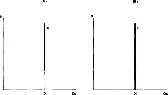
FIGURE 18:

THE EX-POST SUPPLY SCHEDULE.

We should also explain the dashed portion below the lower end of the S schedule in panel A of Figure 18. This indicates the range of relatively low prices at which the firm would not want to sell any of its supply. In contrast, the upper (thickened) portion of the S schedule indicates the range of prices at which the firm would be willing to sell.

Minimum Reservation Prices

Now, what is the difference between the two S schedules in Figure 18? In panel A, the thick portion of the S schedule (as just explained) correlates with those prices on the vertical P scale at which the firm is willing to sell. Hence, the lower end of this thick line indicates the minimum reservation price acceptable to the firm, below which it will not sell. Thus, if market demand is disappointingly low, and buyers would be willing to buy only at the relatively low prices (shown by the dashed portion of S), the firm might decide to withhold the product from the market rather than to sell it at distress prices. In a sense, therefore, the dashed portion shows the prices at which the quantity X would not be offered for sale on the market.

In contrast is the S schedule in panel B, which does touch the horizontal Qs axis. This S illustrates the special but not unusual case where the firm has no minimum reservation price—its goods are placed on sale for whatever price the market will fetch. This includes selling out even at a zero price, which simply means giving the stuff away, with no price asked. Hence, the S schedule is drawn to touch the Qs axis, where P is zero. This means that regardless of the price buyers are willing to pay, firms enter the market prepared to dispose of their wares at any price they can fetch, from zero on up.

Perishables vs. Non-Perishables

A good example of this totally vertical S schedule, which touches the Qs axis, is the perishable commodity (e.g., fish, tomatoes). These commodities may be too costly to store, or not worth preserving, and therefore must be disposed of at whatever price. In such distress situations, the failure of the firm to sell out its supply by the end of the planned sales period puts it under pressure to slash its price sufficiently until it finally does sell out—even if it takes a zero price to get rid of the unsold quantities. In the worst case, where the goods become totally rotten, the firm might even decide to pay a garbage collector to cart the stuff away.

The more usual case involves non-perishable goods—goods that can be stored for long periods of time. Here the seller has an important option: not to sell if the market is not willing to pay his minimum reservation price. This is the case depicted in Panel A of Figure 18. If prices offered are too low, the firm can withdraw its supply and place it in storage. The firm will select this option if it is confident that demand will later pick up sufficiently—sufficiently, that is, to raise prices enough to cover the temporary storage costs. If this speculation fails—if market demand remains weak and the prospect of higher prices fades—the mounting storage costs could eventually induce the firm to sell out at whatever price the market fetches.

Price-setting: Market vs. the Firm

In practice, of course, firms do not enter the market totally ignorant of the prices the market will fetch—without any preconception of the price demanders are willing to pay. On the contrary, firms make appropriate efforts to determine that particular selling price which would enable them to sell their given Qs at the expected profit margin. (This was briefly discussed in Chapter IV, and Chapter IX will deal at length with the relationship between selling price, profits, and costs.) But the point is this: Whatever price the firm initially sets on its product, it must do so with its fingers crossed, because only its eventual confrontation with market demand will determine whether its best-laid plans are successful or not—that is, whether it will be able to sell out its Qs at the original asking P.

In this connection, we shall note that when the S schedule in the graph pertains to the industry as a whole—and therefore represents the market S schedule instead of merely an individual firm’s S—we must be careful how we interpret the lower end of the S schedule (for example, see the S schedule in Figure 19). As we saw above, the bottom tip of the S indicates the minimum reservation price at which the firm is willing to sell. But in the case of the industry or market S schedule, where several firms are involved—each with different costs, profit expectations, and selling prices—we cannot presume to have a single, uniform, minimum reservation price for every firm. These minimum prices will undoubtedly vary from firm to firm. Hence, the lower tip of the S merely indicates the minimum price of only those firms which, for reasons of cost and/or profit margin, are able to enter the market with the lowest minimum prices.

The Marriage of Demand and Supply

We are now prepared to bring both the demand (D) and supply (S) schedules together in the market place—and examine the outcome, as shown in Figure 19. In the nature of the case, we assume that the firms competing in a given market are offering a similar product—as physically similar as is possible in the real world, and as similar as the eyes of the beholders (the consumers) make it.

The first thing to note about Figure 19 is the point E: This marks the intersection of D and S. This intersection point is technically referred to as the equilibrium point, but in simpler terms it represents the market-clearing price ($8 here) at which the total S (the quantity OX) could be sold. That is to say, the point E indicates the only price at which the quantity-demanded (Qd) would be just equal to the Qs—at which the given Qs of X could be sold out in entirety by the end of the planned sales period. This makes the equilibrium price a unique price—indeed, any other price would not have this fortunate market-clearing result, as we will see in a moment.

First, it should be realized that, since different firms are likely to open with somewhat different initial prices for the same product, the market-clearing price of $8 will not necessarily satisfy each firm to the same degree. Only those firms that opened up with an $8 price would discover they were able to sell out within the planned sales period they had set for themselves. On the other hand, those firms that had opened up with prices higher or lower than $8 would experience a different result, technically referred to as “surplus” and “shortage,” respectively. Let us now see how and why.

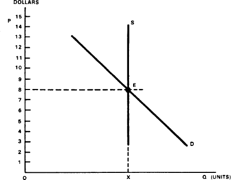
FIGURE 19:

DEMAND, SUPPLY, AND MARKET-PRICE

The Case of a Market Surplus

Assume that, instead of opening up at the happy market-clearing price of $8, the firms had all opened at a higher price, say $11, as shown in Figure 20. Clearly, this $11 price is higher than the market-clearing $8 price. Now, under the law of demand the Qd at $11 will be less than at $8—that is, Qd will drop from OX to OA, as seen along the Q axis. But, since total market S offered is the amount X, the firms now face what is technically called a surplus or “excess supply”: the Qs is of the amount OX, while Qd is only OA. The size of the surplus is indicated by the quantity AX, exactly the horizontal distance by which Qs exceeds Qd at the price of $11.

Let us make sure that we understand why the surplus has occurred. The reason is that at $11 the goods are over-priced, that is, what was a happy price at $8—where Qd was equal to Qs—becomes too high at $11. As a consequence of the too-high price, firms will discover that by the end of the planned sales period—during which they had expected to sell out the quantity X—they are still stuck with an unsold quantity AX. Indeed, well before the end of the sales period, firms will begin to sense that something is going wrong—that their goods are not selling as fast as they had planned. This disappointing rate of sales causes the eventual surplus.

The Case of a Market Shortage

So far we have seen two possible pricing outcomes—one, the happy market-clearing price ($8 here), the second, the too-high price ($11) which caused the surplus. Now we come to a third possibility: the too-low price which results in what is technically known as the shortage or “excess demand.” This is illustrated by the $5 price in Figure 20. At this lower price, the Qd will, of course, be greater than at $8 or $11, but since the Qs being offered is still the same amount X, the result is that Qd exceeds the Qs at the lower $5 price. The size of the shortage is shown by the quantity XB, exactly the horizontal distance by which the Qd exceeds the Qs at the price of $5.

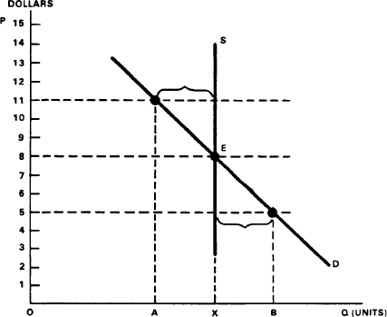
FIGURE 20:

SURPLUSES, SHORTAGES, AND SELLING PRICES.

Again, let us be clear why the shortage emerges. The reason is that, at $5, the goods are under-priced—set below the market-clearing level. This is readily apparent when we compare this outcome with the market-clearing that occurs at the happy price of $8, and the surplus caused by the $11 price. Having set a too-low price, firms will discover that they will have sold out well before the end of the planned sales period. Indeed, they would very early have noticed that their goods were selling at a faster rate than anticipated, which could even make them confident of selling out their supply before the end of the planned sales period.

“Shortages” vs. “Scarcity”

At this point, we should digress to explain the important distinction between a “shortage” and “scarcity.” In these days of politically-generated shortages in oil and other major commodities, it is important to avoid confusing these two terms. Scarcity, as we saw in Chapters I and II, is and always has been a natural condition of human existence—we live in a world which does not have enough resources to satisfy everyone’s wants. As far as economics is concerned, scarcity can never be eliminated—it can only be alleviated. And the only way to alleviate scarcity is to increase production. It is quite otherwise with shortages.

When it comes to shortages, we are dealing with a purely man-made mess, which can be caused by either of the following actions: (1) by setting a too-low price for a given quantity supplied (as we saw in Figure 20, when a price of $5 was set for the quantity X supplied), or (2) by reducing the Qs on the market while keeping prices at former levels. We are already acquainted with the first case; the latter case is best illustrated by means of Figure 21, which is indeed applicable to OPEC’s oil embargo or supply restriction.

How to Create a Shortage

Let us see how Figure 21 illustrates the OPEC policy of restricting oil supply and raising oil prices in order to increase their total receipts (TR) and profits. Assume that the pre-restriction situation is depicted by the quantity-supplied (X) and the price ($3). Clearly the $3 price had been clearing the market of the quantity X. Now comes the restriction of oil supply, indicated by the shift of S to S’ (i.e., from quantity X to quantity A). With this also comes the price increase. But then the question arises: How high can OPEC raise the P? Our diagram tells us that with the given D schedule and the new reduced S’ schedule, P can go up to $11, at which there is a new intersection of D and S’, indicating a new market-clearing P. Not only can P go up to $11, but TR, too, will apparently increase, because (here’s the rub!) the D is inelastic.

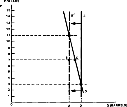
FIGURE 21:

SUPPLY RESTRICTION AND SHORTAGES.

Now, where does the shortage come in? The shortage occurs as soon as suppliers fail to raise P all the way to $11 at the same time that supply is reduced to S’. That is to say, if P stays at $3 or remains at any P below $11, a shortage will emerge! How? First let us see what would happen if the P is held down to $3. Clearly at the $3 price, the Qd will be at X, but since Qs had been reduced to quantity A, there will emerge an excess demand (i.e., shortage) amounting to AX. Now, what would happen if suppliers let P rise to, say, $7? At a $7 price, the Qd will drop to quantity C, but since Qs had been cut back to quantity B, there will still be a shortage amounting to the quantity BC, albeit a smaller one than AX. Only the $11 price would be sufficiently high to erase the shortage and clear the market.

To conclude this digression: Regardless of whether the shortage is initiated by (1) setting a too-low price for a given Qs, or by (2) reducing the Qs but keeping the price below the market-clearing level, the underlying cause of the shortage is, in effect, the same: the selling price is below the market-clearing level and therefore too low in the given demand and supply situation. It follows, therefore, that the shortage could be liquidated in jig time simply by raising the price to a new market-clearing level. Conversely, so long as the price is kept below the new market-clearing level, the shortage is sure to persist.

Surpluses and Shortages are Man-made

Now, to return to our main line. The reader may think it very curious, indeed, that one and the same quantity X supplied by firms could generate three different outcomes—either “shortage,” “surplus,” or “market-clearing”—simply by setting three different prices. But this is precisely the point: for any given quantity of goods offered on the market there is only one market-clearing price—indeed, there never need be a “surplus” or “shortage” so long as price is set at the market-clearing level.

To put it another way: In a world of universal scarcity there is no such thing as an absolute surplus; “surplus” can emerge only relative to a price being set too high. Similarly, when it comes to shortages; scarcity is something that always exists, but shortages arise only relative to a price being set too low. To repeat: For any given Qs on the market, a market-clearing price is the only thing needed to avoid a surplus or shortage. Whereas “scarcity” is the natural condition of human existence, “shortages” and “surpluses” are primarily man-made conditions.

The Planned Sales Period

This brings us to an important question: Which of the three possible outcomes—surplus, shortage, or market clearing—would the firm prefer to experience? Before we answer this, we should first recall something about decision-making in the ex-ante. In Chapter IV we saw that the firm faces the prime task of determining the selling price and the quantity of production that will enable it to realize the desired profit rate—a task made all the more difficult because of the uncertainty of consumers’ demand and the competitive environment. Hence, the firm is incapable of knowing in advance exactly what the market-clearing price will be. In addition to ex-ante ignorance, we should note a few things about our concept, the “planned sales period,” used several times in the preceding analysis.

The planned sales period (PSP) is that period of time by the end of which the firm expects to sell out the quantity supplied to the market. The PSP will vary from product to product, firm to firm, and season to season. Since no firm has an exact pre-knowledge as to precisely how long it will take to sell out its supply—let alone whether it will be able to realize its price and profit expectations—it can only make a best estimate as to the desired length of the sales period and the rate of sales progress. It can then compare the actual rate of sales with the planned, desired rate, and gauge its sales progress accordingly.

Indeed, given the firm’s natural state of incomplete knowledge of market demand—that is, its ignorance of those market parameters affecting selling prices, quantity-demanded, and profit rates—the only alternative guide for measuring the rate of its sa-les progress is its PSP. The PSP at least enables it to judge whether or not sales are moving at the desired rate—that is, the rate that reflects the firm’s best judgment, inadequate as it may be. From this experience—and this experience alone—the firm will be able to learn lessons as to what went right and what went wrong, and improve its ability to plan the next round of production and the next selling program. With this background we can now undertake the task of evaluating the surplus, shortage, and market-clearing outcomes.

Evaluating the Surplus Case

Let us first evaluate the surplus case. Remember: a surplus is the result of a too-high price, which reduces the Qd relative to the Qs. Indeed, even before the end of the PSP the firm will have noticed that its goods are not moving as fast as anticipated. Clearly, the surplus is a disappointing outcome in that the firm must slash its too-high price sufficiently—for example, to $8 in Figure 20—in order to sell out the unsold quantities under the given demand condition. This means that profits will be less than anticipated, and even losses may be incurred.

Furthermore, the firm will face a difficult decision as to how to adjust to the revealed market condition. Specifically, for the next time around, it must either cut its price—and hence its profit rate and/or cost of production—or produce less at the higher price. Either alternative may involve difficult adjustments for the firm, as we will see below.

Evaluating the Shortage Case

What about the shortage case? If you recall, this is the case where the Qd exceeds the Qs because the firm set a too-low price. As a consequence, the firm discovers that its goods sell at a faster rate than expected, so that its supply sells out even before the end of PSP. At first glance this seems to be a happy outcome, not marred by any disappointment. After all, the firm manages to sell out its total Qs at the planned price—and faster than it expected, to boot. What could be better? Upon close examination, however, we find reason for disappointment: the firm could have done even better. Let us see how.

If we assume firms prefer greater profits to smaller profits, it is clear from Figure 20 that, other things being equal, our firms could have sold out the same quantity X at a higher price than $5—indeed, at any price up to $8 they would have been able to clear the market. The reason is that with the given state of demand, any price up to, but not including, $8 induces a Qd greater than the Qs at that price. That is, any price between $5 and $8 would have induced sales to run at a faster clip than expected, and supplies would have sold out before the end of the PSP. Since any price higher than $5 (up to $8) would have meant greater profits, the firms clearly missed a preferred opportunity by selling out at only $5.

The Lack of Advance Knowledge

It is clear that if the firms had known in advance that their initial prices were too low, they would surely have set prices higher than $5 in order to earn higher profits. Having failed to do so, they end up with profits being smaller than otherwise. And the firms have no one else to blame but themselves; they could have detected very early that their goods were selling at a faster rate than anticipated. Then and there they could have begun to increase their prices and watch carefully the extent to which the higher prices slowed down the rate of sales. If worse came to worse, they could always revert back to the $5 price they were happy to start with. Other things being equal, their failure to take advantage of market demand is surely a disappointing experience.

Another disappointment stems from the fact that the firms could have sold a larger quantity (OB) instead of the smaller quantity OX originally produced. That is to say, even if the firms had good reason not to raise their prices above $5—seeking public goodwill, say, or seeking to break into the market by means of this low price—it is clear they underestimated the quantity demanded at the $5 price. This means their sales period ended with some unsatisfied customers—those who came to buy only after the bargain-priced supply had already been snatched up. If only the firms had known in advance that at the $5 price they could have sold quantity OB instead of only OX, they would not be as disappointed as they are now. And who knows if the disappointed customers will ever come back again to see if a new supply is available?

Guessing the Right Price

Compared to the surplus and shortage cases, the market-clearing case clearly must be judged as the preferred outcome: it alone has no disappointment attached to it. That is to say, things work out just as planned whenever firms sell out their supply by the end of the PSP. This is proof they have estimated the market-demand situation perfectly—picking exactly the right price for selling out the given quantity supplied. All of this brings us to another key question: If market-clearing is the preferred objective of the firm—because it marks the perfect meshing of ex-post sales experience with ex-ante pricing and production plans—what prevents the firm from setting a market-clearing price every time? What prevents the firm from realizing in the ex-post its profit-maximizing plans of the ex-ante? What kind of knowledge would the firm require in order to be able to avoid the less-preferred outcomes of surplus or shortage?

Uncertainty and Market Information

The answer to this question was, in essence, already given in earlier chapters. In the real world, the perfect or complete information required by the firm in order to realize its maximizing goals is simply not available to it. Even trial-and-error experience, whereby the firm learns the extent to which it has overpriced or underpriced a particular product at a particular time, does not provide information of a lasting quality. Lessons learned from yesterday’s sales experience do not guarantee success for tomorrow’s sales. The reason lies in the uncertainty and unpredictability of changing market demand: there are continuous shifts in demand schedules (Chapter VI) as well as changes in price elasticity of demand (Chapter VII).

Only in a world in which market demand never changes—in which tastes, incomes, and expectations are constant, and demand schedules do not shift or change their degree of elasticity—only in such a purely imaginary world would today’s demand be the same as yesterday’s, and tomorrow’s the same as today’s. Only in such a make-believe world of no change could firms reasonably expect that tomorrow’s P and Qd would be a mere repetition of today’s. In such a world of repetition and certainty there would be no obstacles to acquiring perfect knowledge of the market demand—and trial-and-error search for the right price and quantity would become unnecessary! But a world of certainty is a pure figment of the imagination, useful only for the purpose of explaining why in the real world perfect knowledge is impossible.

Market as a Feedback Mechanism

It follows, therefore, that in the face of changing market demand, it is not logical to assume that firmis it logical to believe that any other group of people possesses such complete information, be they economists, consumer advisers, or politicians. The best that the firm can do is to arrive at approximate knowledge of the market—knowledge that reduces the areas and degrees of its ignorance. Approximate knowledge is the only kind of knowledge available to man—obtainable only from daily trial-and-error in the market—and trial-and-error experience is the only kind available.

Thus we can now see that the occurrence of surpluses and shortages is precisely the market’s way of informing the firm that its plan has fallen short of the mark, and that it must henceforth make adjustments in price and/or quantities the next time around. In a moment, we will analyze these adjustments to market surpluses or shortages. Suffice it to emphasize here that the market is the only feedback instrument available for signalling to the firm that its price is not right, and that it had better change it.

Guessing the Right Quantity to Supply

This brings us to another crucial aspect. Not only does the market provide feedback signals to the firm when the selling price is not right, but it also sends up signals when the quantity supplied is not right—signals that likewise take the form of surpluses or shortages. Decisions by firms can result in surplus or shortage not only when they set prices too high or too low, but when they produce quantities that are too large or too small, relative to the selling price. This can be readily seen with the aid of Figure 22.

Now, in Figure 22, it is assumed that all firms are selling the same product at the same price of $8. On the other hand, it is assumed that different firms may produce different quantities. For instance, the market outcome is vastly different when firms produce excessive amounts—on the “surplus” scale OB, say—compared to when they produce the relatively modest quantities on the “shortage” scale OA. There is also a third possibility—when firms produce on the scale of OX, which we will see is the market-clearing case. Let us examine each of these cases in detail.

When Firms Produce “Too Much”

First, why does the supply schedule Sb in Figure 22 represent a surplus case? Because the firms have produced a quantity (OB) that exceeds the quantity-demanded (OX) at the common $8 price—clearly they have overestimated the Qd at this price. As a consequence, they discover fairly early that their product is not selling as fast as expected, and at the end of their planned selling period they are stuck with a pile of unsold goods.

Had the firms been equipped with perfect knowledge of the demand situation, this surplus could have been avoided in either of two ways. First, the firms could have offered the smaller quantity OX (Schedule Sx). The OX quantity would have cleared the market, since at the $8 price the Qd and Qs are exactly equal, as indicated by the intersection of demand (D) and supply (Sx). Alternatively, the firms could have avoided surpluses by selling the quantity OB at the lower price of $5, which, indeed, is a market-clearing price for the given quantity supplied: at this price the Qd (OB) is exactly equal to the Qs (OB). In the absence of perfect knowledge, however, the firms were ignorant of both the market-clearing price (given the Qs) and the market-clearing quantity supplied (given the P).

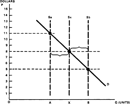
FIGURE 22:

SURPLUS, SHORTAGE, AND QUANTITIES SUPPLIED.

When Firms Produce “Too Little”

Next, why does the supply schedule Sa in Figure 22 represent a shortage case? Because while the firms are producing quantity OA, the Qd at the price of $8 exceeds the quantity being supplied by the amount AX. It is apparent that the firms undershot the mark: they underestimated the demand at the $8 price. And they could very early have spotted signs of the impending shortage: they could have noticed that the actual rate of sales was exceeding the expected rate of sales.

Had firms known in advance exactly where the market demand schedule was located, they could have resorted to more profitable alternatives. For one thing, they could have planned to produce the larger quantity OX (instead of OA), which would have cleared the market at the original $8 price. (This can be seen by the intersection of the Sx schedule and the D schedule at the $8 price.) On the other hand, the original output of OA (schedule Sa) could have been released at the higher price of $11 (instead of $8), and still clear the market, since at $11 the Qs would have been exactly matched by the Qd.

A Backward Glance

Before we proceed to examine how firms can adjust to the market’s feedback signals—that is, to surpluses, shortages, or market clearings—we should briefly review the ground we have covered.

For any given quantity supplied by the firm, the problem becomes one of setting the right price—the price that will clear the market within the planned sales period (PSP). Otherwise, if it sets the P too high or too low, the result will be either a surplus or a shortage, respectively. Similarly, for any given price at which the firm wants to sell, the problem becomes one of gauging the right quantity to produce in order to clear the market. Otherwise, if it produces too much or too little, it will end up facing a surplus or shortage, respectively.

Also, for convenience, we will hereafter refer to a surplus or a shortage as a disequilibrium type of outcome. A “disequilibrium” simply means that, for the time being, the firm has failed to achieve its market-clearing or equilibrium objective within its PSP, and that it therefore faces a decision: What to do about disequilibrium?

III. How Firms Adjust to Market Conditions

By now it should be obvious that the firm’s adjustments to market disequilibria can involve changes in its selling price (P) and/or quantity-supplied (Qs). Altogether, the firm can make three possible adjustments: (1) change its selling P, or (2) change its Qs, or (3) make a combination of changes in both P and Qs. Thus, in response to disequilibrium, the firm might institute a cut (or increase) in P, or a reduction (or increase) in Qs, or some combination of changes in both P and Qs.

Current Adjustments vs. the Next Time Around

Now, all of these adjustments can take place in either of two different time phases. One type of adjustment may be termed a current adjustment. As soon as the firm senses that its current sales are deviating from the planned path—that they are progressing at a faster or slower rate than planned—the firm can immediately change its P and/or Qs in order to improve sales or minimize disappointment before the end of the current PSP.

The second type of adjustment is not made currently but is delayed until the next time phase—the one following the current sales period—which we can term the next-time-around (NTA) adjustment. In this case the firm does not make any current adjustments: for one reason or another, the firm decides to do nothing now about the discrepancy between the actual rate of sales and the planned rate. Instead, it rides out the current period and reserves its P and Qs adjustments for the NTA.

Firms Cannot Rest on Their Laurels

None of this implies that an NTA adjustment in P and Qs is required only in response to a disequilibrium outcome. That is, it does not imply that a happy market-clearing experience will never induce the firm to make a subsequent NTA adjustment. In free competitive markets no firm can afford to rest on its laurels—even when it enjoys a market-clearing experience. Market conditions are in constant flux, and changing demand is a constant source of uncertainty. Yesterday’s success cannot guarantee tomorrow’s success. Successful market-clearing is due more to good fortune—a happy coincidence of objective market conditions and entrepreneurial plans made by the firm—than to any precise foreknowledge of market conditions.

For example, if a firm succeeds in clearing the market as planned, should it merely repeat by producing the same Qs at the same P as before? Can it simply rely on market demand remaining the same as before? Or must the firm be alert to any possible shift in D, or change in elasticity of D? Clearly, in a dynamic changing market, the firm must be on constant alert. Thus it makes no difference whether the firm ends its PSP with a surplus, shortage, or market-clearing—it will always have to face the important entrepreneurial decision for the NTA: What should it decide for its next P and Qs?

Making Adjustments to a Surplus

We are now ready to examine the types of adjustments the firm can make in response to a surplus or shortage. In the case of a surplus, it makes no difference whether it was caused by (a) overpricing a given supply, or (b) overproducing at a given price—the analysis runs along similar lines. For the overpricing case, refer to Figure 20: there we see that the $11 price is too high for the given supply OX, hence the surplus of AX. For the overproduction case, see Figure 22: there it turns out that the $8 price is too high for the supply OB, hence the surplus of XB. In both instances, the basic cause of the surplus may be viewed as overpricing the given supply, or overproducing at the given price. Both instances turn out to be merely two sides of the same coin—an overpriced supply. With this understanding, let us focus on Figure 22 for convenience.

Now, what can the firm do in response to the surplus XB in Figure 22? If the firm spots the surplus in its incipient stages, during the current sales period—as soon as sales fail to progress at the expected rate—it can decide then and there to slash its current P from $8 in order to step up the rate of sales. However, so long as the reduced P remains above the market-clearing P of $5, some surplus would remain at the end of the PSP. In order to sell out the last unsold unit, the P would eventually have to be cut to the $5 level. On the other hand, if the firm decides to avoid any P-cutting until the bitter end of the PSP, even then the same truth holds: P must at last be cut to $5 in order to clear out the remaining unsold units.

Next-Time-Around Adjustments

So much for current adjustments to the unfolding surplus. What about next-time-around adjustments? What lessons can the firm learn from its bitter experience and apply to its NTA production and pricing programs? One option is to produce the same quantity as before, which means a repetition of supply schedule Sb. However, this would call for a lower price of $5 as against the former opening P of $8.

This raises the relevant question: Can the firm manage to cut P to $5 without squeezing its profit margin? That is to say, can it also cut its costs as well as its P? This brings up a touchy practical problem: since wages are usually the major component of costs, can labor resistance to cuts in wage-rates prevent firms from cutting costs? If costs cannot be cut, will the firm be willing to accept a cut in profit margin?

Cutbacks in Production

A second option is for the firm to retain its former opening P of $8 but, instead, reduce its Qs to OX (schedule Sx), which, too, would be a market-clearing program. This would obviously call for a reduced rate of production and supply. Assuming that the reduced rate of production does not significantly affect the cost-per-unit of product, this cutback in output would not affect the margin of profit between selling P and cost-per-unit of product. Nevertheless, cutbacks in production could also mean layoffs and reduced employment, which may be as distasteful to workers as cuts in wage-rates.

The first two options give rise to a third option—a combination of both price and production adjustments in the appropriate direction—that is, a combination of price-cut and production cutback. More specifically, P could be cut to somewhere between $8 and $5, while Qs would be cut to somewhere between OX and OB (i.e., between schedules OX and OB). Technically speaking, any “dot” on the demand schedule in the segment located between the $5 and $8 P would yield a P and Qs combination capable of satisfying this adjustment.

Withholding Supply and Speculation

Since price-cutting can be bitter medicine, the firm may prefer a more palatable alternative: avoid any P-cuts but, instead, withdraw the unsold quantities from the market and withhold them until demand increases sufficiently to clear the market at the original price of $8. (Technically speaking, the expected increase in demand would be depicted in Figure 22 by a shift of D to the right, to the point where it intersects Sb at the $8 price.) However, withholding of supply from the market involves speculation; it is based on the expectation that the future holds a desirable market change in store. In the present case, the firm speculates that future demand will be sufficiently greater than today’s; this would make it preferable to sell tomorrow at the desired $8 price rather than to sell out today at a lower price.

However, the withholding of supply for speculative purposes is not without cost. One speculative cost is the cost of warehousing the withheld quantities. Second, there is the uncertainty of how long the firm will have to wait until demand increases sufficiently. In the worst case, demand may not increase at all. In any event, the fact remains that withheld supplies constitute unsold products, and until demand increases sufficiently, the firm is haunted by a dilemma: to withhold or to sell out at slashed prices. Which will minimize its losses?

Which of these options should the firm resort to? Only the firm itself can decide which course is best. Economics as such is not capable of foretelling which course of action would be taken by any particular firm in a given circumstance. All it can say is that whatever adjustment the firm decides upon will be a maximizing decision, albeit in the given circumstances designed to minimize losses resulting from the surplus.

Making Adjustments to a Shortage

We now turn from the surplus case to the case of shortages. How can the firm adjust to a shortage outcome? (The shortage is depicted in Figure 22 by the Sa schedule and the $8 price, which together yield a shortage amounting to AX.) In contrast to the surplus case, the shortage generally poses fewer difficulties or dilemmas for the firm. Other things being equal, a firm would rather sell its product at a faster rate than at a slower rate. Nevertheless, the firm does face a tantalizing decision as soon as it notices that its sales are moving at a faster rate than planned. It then realizes that its goods will be sold out well before the end of its PSP—and that there will remain unsatisfied customers as long as the price is kept at $8 while Qs is not increased. Clearly, the firm had underestimated market demand, which turned out to be OX, whereas it had produced only OA. What type of current adjustment should it now make?

For one thing, firms could decide to immediately raise their current price—indeed, according to Figure 22, they could raise P to $11 and still sell out their total supply of Sa. But would they feel entirely at ease raising the P in order to take advantage of market demand being greater than anticipated? Would they feel uneasy or hesitant about bucking widespread social pressures and taboos against “charging what the traffic would bear”?

On the other hand, if they decide not to raise their P—in order to curry public goodwill, say—they would be foregoing an opportunity to increase their profits. Could they nevertheless compensate by stepping up the rate of supply by dipping into inventories in their warehouses? In this way they could release increased Qs to the market, reduce the number of unsatisfied customers, and increase their total profits. But would this dipping into inventories be enough to quench the unsatisfied demand?

Utilization of Existing Facilities

If firms do not raise prices, and inventories are depleted before the shortage is eliminated, they may still have an ace up their sleeves: more intensive utilization of their existing productive facilities.

It is not at all unusual for plants to be operating at less than “full capacity.” Indeed, by design, most plants are built to scales larger than would be required by the average rate of sales anticipated by the firm. This oversizing of plant provides elbow room for the firm—a margin of extra productive capacity—which it can lean on if and when demand proves to be larger than anticipated. The shortage case here calls forth such an instance. If a shortage arises while firms are operating at, say, only 75 or 80 percent of rated capacity, then they have a margin of capacity that can be utilized to increase their Qs in the NTA.

The problem here, however, involves a crucial economic fact: if the plant is already at a high rate of utilization (say, 85 percent or more), a further increase in the rate of plant utilization would be associated with an increased cost for each unit produced. The reasons for this increase in unit or average cost (AC) are multifold.

For one thing, the extra production load may involve overtime labor at extra overtime rates of pay. Also, there may be additional expenses due to breakdowns in overworked equipment and the resultant bottlenecks. Then, additional workers may have to be hired, but since they are not likely to be as efficient as the regular labor force, their labor will not be as productive and their output will cost more per unit. All this adds to the average cost of the product, with the consequence that the firm has to ask for a higher price for its product.

Price Inducement and Imports

Even with a more intensive utilization of existing productive capacity, the stepped-up rate of output may not be enough to overcome the shortage. That is to say, the industry supply schedule may not be able to shift enough to the right, to where it coincides with Sx in Figure 22. If so, as long as the Qd continues to exceed the Qs and the shortage persists at the existing selling price of $8, this price would be under pressure to rise.

As a matter of fact, this rise in P is precisely what the doctor would order: it induces firms to step up their rate of plant utilization since it compensates for the increase in average cost of output. Otherwise, the necessary margin of relief might have to come from imports of goods from other countries. But the flow of imports depends essentially on the ability of foreign producers to sell at prices competitive with domestic producers, unimpeded by legal trade barriers such as tariffs and quotas.

The Next-Time Around Problem

Whatever the firms decide to do by way of current adjustment, they are still faced with a next-time-around adjustment. Here the problem facing the firm is no less ticklish than in the previous case. One option we have already seen: raise the price next time to $11 while producing the same amounts as before. Assuming that demand will stay the same, the total supply will still clear the market even at the higher P. After all, that’s what the D schedule in Figure 22 says: at any price less than $11 the Qd will exceed the Qs. Hence, as long as P is not raised to $11, the firms will be fostering a shortage. Now, the main problem with raising price is whether firms can either (a) suppress their collective fear of the public wrath against charging what the traffic will bear, or (b) make public opinion more hospitable to the idea that firms have a right to charge whatever price the public is evidently willing to pay.

Increasing Supply by Capital Investment

If firms prefer to leave the price as is, at $8, they can resort to another NTA adjustment: increase the Qs from schedule Sa to Sx. This would enable firms to eliminate the shortage by an expansion of supply. The increased number of units sold would result in increased total profits even though the profit rate per unit sold would remain the same as before: since the P remains unchanged at $8—and we are assuming the cost per unit of output is also unchanged despite the higher rate of production—the price spread between P and average costs remains the same as before. (Review Chapter IV on the “price spread.”)

The main problem with increasing the Qs while holding P the same is that the expansion of output will involve capital investment of the type discussed in Chapter IV. As we saw there, expansion of output might require increased scale of plant operations, which, in turn, involves acquisition of additional machinery and space as well as hiring more labor. These expenditures, in turn, would require additional financing from internal sources—such as profits and depreciation allowances—and/or external funds from the money and capital markets.

Once Again: Uncertainty and Risk

Underlying the investment decision, of course, is the assumption that the firms know exactly by how much their Qs should be increased. But such an assumption is too glib. It is one thing to play around with diagrams like Figure 22, from which it is readily seen that Qs should be increased from OA to OX, which would still clear the market. But in the real world it is not so easy to discover where the new market-clearing supply schedule lies. Uncertainty of demand makes it virtually impossible for firms to predict the location and slope of D in the NTA period, and therefore creates considerable risk in the investment in enlarged productive capacity. In any event, the fact remains that as long as the Qs is not increased sufficiently, the shortage will persist—which is, again, the market’s way of informing firms that sales opportunities still remain.

As we conclude this portion of the chapter, let us pause once again to see how we can reach some simple conclusions despite the possibly confusing details of the complex analysis. After all is said and done, the following simple truth remains: however the firm decides to adjust to uncertainty of market demand, this adjustment always boils down to determining, as best it can, that particular combination of P and Qs that will clear the market. Still, so long as the market fitfully turns up surpluses or shortages, the firm’s adjustment problems remain. Indeed, even when it succeeds in clearing the market as planned, such success is but a fleeting fortunate outcome—the firm has no cause to rest on its laurels in a world of seething uncertainty.

IV. The Law of Market Price

We are now at the point where we can assert the key proposition of this chapter, the Law of Market Price: in a free market unhampered by government price-fixing or other market interventions, the selling prices set by firms will tend to move toward the market-clearing (“equilibrium”) level, where the quantity supplied equals the quantity demanded at that price.

As a corollary to the law of market price we should add: any other price, higher or lower than the market-clearing price, would cause disequilibrium situations such as surpluses and shortages. Since these outcomes would be considered by firms as less than optimal compared with market-clearing prices, firms in the free, competitive market will be motivated to avoid or minimize them by appropriate price and quantity adjustments.

More on the Free Market

The free market will be discussed in detail in Chapters X and XI. Here it will suffice to note the following. In addition to the introductory remarks at the start of this chapter, the term “free market” includes the following two characteristics about firms. One is that firms are motivated primarily to make profits (and avoid losses), and to increase their total wealth in the interests of stockholders, while keeping non-monetary goals to a minimum. Thus, we exclude nonprofit organizations from this context.

The second feature is this: firms have to make it strictly on their own—without paternalistic protection from government in the form of minimum prices, subsidies, bailouts, tariffs, or guaranteed markets. This implies that firms must earn their profits purely by their own ability to cater successfully to consumers, and that they will suffer losses for failure to meet consumers demands satisfactorily. As a consequence, firms will be strongly motivated to maximize profits and minimize losses.

“Supply Equals Demand”?

Next, let us be technically clear about the meaning of market-clearing price: it is the price at which “Qs equals Qd”—which is not the same as saying “supply equals demand.” These are two totally different expressions. The latter expression is unquestionably the more popular, especially among people who are not sophisticated in economics. Yet, it is simply not correct to say, “S equals D” in the present context.

To be precise, “S equals D” literally is an absurdity. As stated, it implies that both S and D schedules are superimposed upon each other, which in turn means that at every price the Qs equals the Qd. This is an impossibility: ex-post supply schedules are vertical, whereas demand schedules slope downward from left to right; this permits only one point (i.e., the intersection point) at which the Qs equals Qd. That is, there is only one price at which there can be equality of Qs and Qd and market-clearing; at all other prices there is discrepancy between Qs and Qd, not equality. In contrast, the statement “S equals D” implies that, since Qs equals Qd at every price, there is market clearing at every price! Clearly an impossibility.

The Tendency to Market-Clearing

Also notable above is our statement that selling prices will tend toward the market-clearing level, and need not hit the mark every time the firm sets it price. Despite the firms’ lack of perfect knowledge of D and S conditions, they are motivated to seek market-clearing outcomes and avoid disequilibrium outcomes.

For one thing, there is the economic incentive to maximize profits. As we have seen, surplus and shortage outcomes cause the firm less profit than otherwise under the given D and S conditions. Thus, in the case of a surplus, the firm will have to slash its P below the planned level, whereas in the case of a shortage the firm has missed an opportunity for greater profits by setting its P too low or producing less than the market was ready to absorb.

On the other side of this coin is the fact that, of the three possible market outcomes—market-clearing, surplus, or shortage—only market-clearing outcomes validate the firm’s expectations and strengthen its confidence in its ability to judge market conditions. In contrast, surpluses and shortages are truly disappointments—sources of regret and diminished confidence.

What About Disequilibrium?

This brings us to the word optimal, which characterizes the market-clearing outcome. “Optimal” signifies that the firm’s ex-post experience most nearly approximates its ex-ante expectations, and, hence, minimizes disappointment and regret. In effect, therefore, the law of market price says that, as long as firms are motivated to optimize the relation between ex-post experience and ex-ante plans, selling prices will tend to be market-clearing rather than disequilibrating.

Before we proceed, we should note that not all disegulibrium outcomes can be blamed on the incomplete knowledge of the firm and its planners. As we will see in the next part, surpluses and shortages also occur as a result of independent shifts in market demand and supply—that is, demand shifts caused by changes in tastes, income, population, or price expectations (see Chapter VI), and supply shifts caused by the vagaries of nature (e.g., bad crops caused by bad weather) or government policies (e.g., wheat price-fixing or oil supply restriction). While such disequilibria are not the direct result of decisions by the firm, they nevertheless exert significant impacts on profits and sales opportunities, and the manner in which the firm responds to them can determine its prosperity and growth.

Government Interventions and Non-Profit Pricing

As we have indicated, because of uncertainty and ignorance, firms will experience shortages and surpluses about as often as market-clearing. In a free market, such disequilibrium outcomes would tend to be short-lived or temporary. However, if and when the surpluses and shortages become persistent or long-lasting—a situation thoroughly inconsistent with free-market conditions—the cause must be sought elsewhere: (1) in government price-fixing or other interventions, and (2) non-profit pricing policies. This is not the place for a detailed analysis of government policies affecting the free market; they will be briefly discussed in Chapter X. “Non-profit” pricing by private organizations such as colleges, theater companies, and civic groups will be discussed here briefly.

Non-profit organizations include groups like the Rose Festival Association—which, with its affiliated colleges, produces the annual Rose Parade and Rose Bowl game—as well as opera associations, and virtually all fraternal and religious organizations. These organizations differ basically from profit-seeking corporations in that they, for various reasons, do not seek to sell their products or services at market-clearing prices—prices that would maximize their profits and wealth. Indeed, they characteristically underprice their goods and services, causing inevitable shortages.

Why Blame the Ticket Scalper?

How can non-profit underpricing by a group like the Rose Bowl Association cause a shortage? Imagine, as in Figure 23, that there is a given supply of football tickets (S) for seats at mid-field, and that the demand for these tickets is great enough to clear the supply (OX) at an $8 price. Now, if the Rose Bowl people decide to sell these tickets at $5 instead, knowing full well they could easily sell out at a much higher price, they are clearly inviting a shortage—shown by the excess demand XB—with all of its familiar symptoms: excessively rapid rate of sales, long waiting lines of customers (queues), and black-market sales by ticket scalpers (since it is illegal to resell tickets at a price higher than paid for). By design, the Rose Bowl people had underpriced their product and, of their own account, brought on the shortage.

Indeed, the much maligned ticket scalper is merely rushing into a good thing when he sees it. The profits that he siphons off for himself could as easily have gone to the Rose Bowl group. Ironically, so-called “non-profit” pricing turns out to be an excellent source of profits for the speculators! Would our imaginary Rose Bowl people but realize that they—by their policy of underpricing—and not the ticket scalper, are responsible for inducing illegal speculation in tickets, they might question the wisdom of their “non-profit” pricing policies. It is proverbial in economics that whenever you spot illegal ticket-scalping or black-market activities, you can smell an underpriced product. It should also be noted that government rent controls and similar price-fixing policies, that characteristically underprice the product, are a prime cause of illegal black markets.

Ticket Scalpers on Broadway

One more example of non-profit underpricing suffices to reinforce our point. For a long time, tickets to Broadway shows had been priced according to arbitrary, traditional, or inflexible formulas rather than by flexible adjustment to demand and supply conditions. As a consequence, it was not unusual to see tickets for different shows selling at about the same price, even though some of the shows were smash hits while others were duds. In a truly free market, prices for the former shows should have been significantly higher than for the latter. In practice, however, even tickets to such classic Broadway smash hits as South Pacific and My Fair Lady were invariably underpriced.1

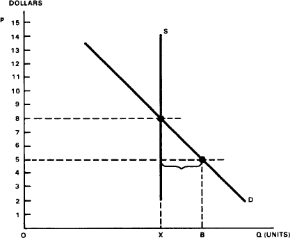
FIGURE 23:

NÒN-PROFIT UNDERPRICING.

The results were inevitable. Induced shortages found ticket buyers scrambling for available tickets, while ticket scalpers, seeing a good thing in the underpriced tickets, moved in to make their profits. In some cases, dollar receipts of scalpers were about two to three times as great as box-office receipts! Indeed, even some of the managers and their box-office people were enticed by the situation and connived with scalpers for part of the latter’s profits!

The bitter irony is that the theaters’ hidebound adherence to underpricing, and their refusal to charge what the traffic would bear, constituted an open invitation to the ticket scalper to play his “evil” role. As a consequence, the profits that were diverted to ticket scalpers could have gone instead to the creative performers and professionals who made the hit show possible in the first place—the actors, musicians, authors, composers, lyricists, directors, and stage hands!

V. When Market Conditions Undergo Change

This final section of the chapter shows how demand-and-supply analysis helps us answer such important questions as: What kind of demand-and-supply conditions cause changes in prices? For instance, what D and S conditions enable or induce P to rise, or pressure P to drop? A related question is: If prices have been rising or declining for some time, what could have caused these price trends? Another group of questions focuses not directly on prices but on the underlying demand and supply conditions as possible cause of future price changes. For example, what will happen to prices and quantities if and when demand and/or supply increase or decrease?

First, Some Diagrammatic Aspects

The analysis will be greatly facilitated by the use of diagrams showing how demand (D) and supply (S) schedules shift—that is, increase or decrease—and how these shifts cause prices to change. We have already seen in Chapter VI (Figure 10) how demand schedules can shift. Now, for the first time, we see (in Figure 24) how supply schedules can shift. Panel A shows a shift of S to the right (from S1 to S2), indicating an increase in S and Qs. Panel B shows the reverse happening, a decrease in S (from S1 to S2) and Qs.

We can now turn to the first set of questions raised above, specifically: Under which D and S conditions could prices rise? We are using the word “could” in the sense of “be able to.” Thus, our question really is: Under which D and S conditions would P be able to increase? This kind of question is typical in the physical sciences, i.e., what conditions would be required in order to enable some particular event to transpire?

Enabling Prices to Rise

Imagine a market that has, up to now, been in a state of equilibrium, with supplies being cleared at the current $6 price (Figure 25). Now, along comes an increase in demand, while supply conditions remain the same as before. The increase in D in Figure 25 is shown by the rightward shift from D1 to D2, while the stationary supply schedule is shown by S at X. Why did demand increase? It could have been a general increase in wages and other incomes, or more intensive tastes, or some other non-price determinant of demand (see Chapter VI). For the sake of illustration, it makes no difference which it was.

Our diagram tells us immediately that the increase in D from D1 to D2 induces an increase in price (P) from $6 to $9. This is indicated by the new (higher) intersection point of the increased D2 with the given S. At the $9 price the market would achieve a new market-clearing situation, in which the Qs once again equals the Qd, albeit it takes a higher price to accomplish it. Thus, higher prices will be associated with an increase in D, as long as S remains the same.

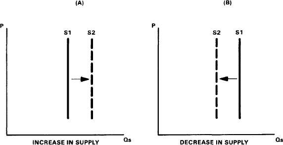
FIGURE 24:

SHIFTS IN SUPPLY SCHEDULES.

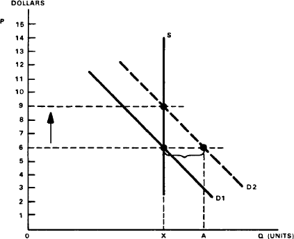
FIGURE 25:

INCREASE IN DEMAND WHILE SUPPLY IS FIXED

We are now able to start answering our first set of questions. For example, under which conditions would sellers be able to increase P? Figure 25 provides at least one answer: whenever D increases relative to S, P will be able to rise. Why? Because, with the increased demand, but unchanged supply condition, the ensuing shortage finds buyers are willing and able to buy the existing quantities X at any P between $6 and $9. That is, any P up to $9 still leaves the market unsatisfied: the Qd remains in excess of the Qs (i.e., a shortage). So long as there are demanders who, under the new schedule D2, are willing and able to pay up to $9, sellers will obviously be able to ask and get the higher P.

A Decrease in Supply

Another situation in which a rise in prices would occur is presented in Figure 26. Here we see an increase in P that results from a decrease in supply—while demand conditions remain the same as before. The decrease in S is shown by the leftward shift in S from output X to A, while the D schedule remains fixed. Again, it is not necessary to know the specific cause of the drop in S—whether it is due to, say, work stoppages by labor unions, or the withholding of supply by producers (e.g., the OPEC oil embargo); it makes no difference for illustration purposes.

It is apparent from the diagram that the drop in supply from X to A induces an increase in P from $7 to $12. The higher P is indicated by the new (higher) intersection point of fixed D with the reduced Sa. Thus, a new market-clearing situation has been reached by means of the increase in P which reduces the Qd to equality with the reduced Qs (OA). Hence, a higher P would be associated with a reduction in S, so long as D remains unchanged.

Why are sellers able to raise P in the case of a reduced S? It is essentially the same shortage condition that arises in the case of increased D—except that now, with the reduced S but unchanged D, there are demanders who are still willing to buy the scarcer quantities (OA) at any P between $7 and $12. That is, any P below $12 would still leave Qd in excess of the Qs, hence shortage. As a consequence, sellers will clearly be able to ask and get higher prices—on up to $12—so long as the reduced S condition prevails and D is fixed in the previous position.

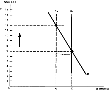
FIGURE 26:

DECREASE IN SUPPLY WHILE DEMAND IS FIXED.

Edging Prices Downward

Let us now skip to the opposite side of the ledger and ask: Under which D and S conditions would prices be under pressure to decline? To answer this question, we go to Figure 27. Here we see that the decrease in P from $8 to $5 is spurred by a decrease in demand, while supply remains unchanged. The decrease in D is illustrated by the leftward shift from D1 to D2, while S remains fixed at output X. The cause of the drop in D might have been a decline in people’s incomes or some other appropriate change in non-price determinants of demand, but it does not matter for our present purpose.

It is readily seen in Figure 27 that the decline in demand calls for a decrease in P from $8 to $5. The lower P, which corresponds to the new (lower) intersection point of fixed S with D2, precisely enables the necessary market-clearing—the equality of Qd with Qs—even though D has dropped while S remains fixed. Thus, the decrease in D is associated with a lower P, so long as the S that needs to be cleared remains fixed.

How do we explain the reduction in P associated with the drop in D? By the fact that if P were not cut, but kept at $8, the result would be an unsold surplus amounting to AX. That is, at the original $8 price, Qs exceeds the reduced Qd. Only the drop in P whittles away the initial surplus, and only when P has fallen to $5 will the surplus be entirely eliminated. If sellers really wish to clear the market of the given S, only the cut in P will do it.

An Increase in Supply

What else could cause prices to be under pressure to decline? Figure 28 tells us that an increase in supply would bring on a decrease in P. The increase in S is indicated by the rightward shift in S from quantity X to A, while the demand schedule (D) remains the same as before. The increase in S could have been caused by an expansion of productive capacity by existing firms, or by the entry of new firms.

Our diagram reveals, furthermore, that associated with the increase in S is a drop in P from $11 to $6. The lower P is indicated by the new (lower) intersection point between the fixed D and the increased Sa. It is the reduction in P which induces the Qd to increase enough to absorb the increased Qs (OA). Thus, the reduced P is associated with the increase in S, while demand remains the same.

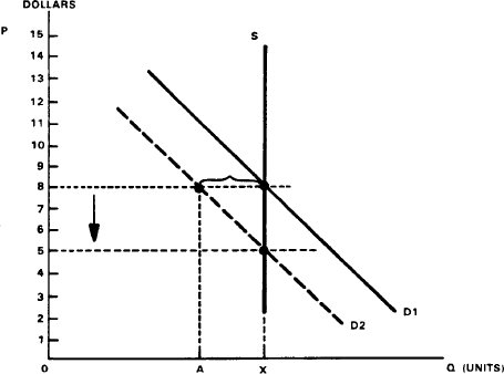
FIGURE 27:

DECREASE IN DEMAND WHILE SUPPLY IS FIXED.

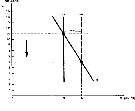
FIGURE 28:

INCREASE IN SUPPLY WHILE DEMAND IS FIXED.

By now it should be easy to explain the connection between the increase in S and the drop in P. It is the same condition of surplus that occurs in the case of reduced D. If P had been locked at the original $11 and not allowed to fall, an unsold surplus (amounting to XA) would have ensued. The $11 price would have left the old Qd far short of the expanded Qs. Only the drop in P induces the increase of Qd that absorbs the initial surplus. Only when P eventually descends to $6 will Qd be equal to the expanded Qs. Clearly, so long as suppliers wish to clear the market of the increased S, only the reduction of P will enable them to do so.

A Brief Summary

By way of review, we can state in general that changes in prices result from changes in demand or supply—from shifts in the D or S schedules. Furthermore, the preceding analysis enabled us to kill two birds with one stone. It not only showed how changes in demand and supply conditions affect market prices, but it also revealed a new source of disequilibrium. In earlier parts of this chapter we saw how firms themselves could cause surpluses or shortages by overpricing or underpricing, and by overproducing or underproducing. Now we see that changes in the market—shifts in D or S—can initiate surpluses or shortages.

Long-Run Decline in Prices

We are now prepared to see how demand-and-supply analysis enables us to locate the basic forces behind historical price trends. For instance, we know from the history of the 19th century that the U.S. experienced a general downward trend in prices through most of the century. The only exceptions to the secular decline in prices came during periods of war and economic boom. Compared to the almost uninterrupted inflationary price trend since World War II—in the U.S. as well as in major Western countries—the 19th century deflationary trend looms as a truly remarkable event. And yet it can be readily explained by economics. How?

For clues to what could have caused the overall decline in prices, we can refer to our preceding analysis. One possible clue, diagrammed in Figure 27, is decreasing demand, which by itself could cause P to drop. But such a decrease in D cannot really serve as an explanation because D actually increased on a vast scale during the 19th century—and an increase in D itself would cause P to rise. However, since we also know that supply increased greatly during the 19th century, a more likely explanation is to be found in Figure 28: this shows prices crumbling under the pressure of expanding supply, a fact that obviously corresponds much more with 19th century experience than declining D. Indeed, the expansion of S was so great, especially after the Civil War, that it must have more than offset the effects of the long-run expansion of D. By itself, an increase in D would induce an increase in prices, but when it is accompanied by an even greater increase in S, the net effect is to cause a downward trend in P. This combination of forces is depicted in our new Figure 29.

Diagrammatic Aspects

First, notice the overall decline in prices over the long run, as indicated by the dashed line. Also notice the faster rate at which the S schedules increase compared with the increase in D schedules. For example, by the end of the second period, supply has reached the S2 position, whereas demand has only increased to the D2 position, so that D2 intersects with S2 only at a lower P. And so on. As a result of S generally running ahead of D, the successive intersection points between them come at lower and lower levels of market-clearing P. The reason is that, at previous prices, Qs exceeds Qd; hence, the faster-increasing S could be absorbed only at falling prices. Alternatively, the increased productive capacity and efficiency of the economy enable successive cuts in prices.

In Figure 29 we also have a diagrammatic novelty. For the first time, we show both demand and supply schedules shifting simultaneously. This is the more realistic case compared with the above cases in which only one schedule shifted while the other schedule stayed fixed. Indeed, this diagram illustrates a general proposition that follows from our preceding analysis: whenever the rate of expansion in S exceeds the rate of increase in D—based on increased productivity and lower costs—prices will decline because of the pressure of excess S relative to D.

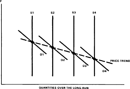
FIGURE 29:

LONG-RUN DECLINE IN PRICES.

Long-Run Rise in Prices

Supply-and-demand analysis is also useful in explaining the long-run upward trend in prices, popularly referred to as inflation. For instance, ours has been called the “Age of Inflation,” denoting the fact that prices have been rising more or less steadily in the U.S. and other major industrial countries since the 1930’s. Indeed, inflation has become the predominant long-term problem of our times, which makes it an important subject for analysis. However, inflation would take us beyond the scope of the present work. Suffice it to say that, in spite of protestations to the contrary by many people who claim that modern inflation is something “new,” and as yet without a solution—as though it were a mysterious visitation from a remote planet—the fact remains that the cause of inflation can be described simply in demand-and-supply terms. Let us now see how.

First, let us check out one possible explanation for rising prices in the U.S.—a reduction in the supply of goods. (This was diagrammed in Figure 26.) True, a continuous drop in S in the face of sustained D would, by itself, cause P to increase. But this possibility is disqualified as an explanation of modern inflation because, at least for the period since World War II, the U.S. enjoyed undoubted expansion of S (not contraction). And as we know, an increase in S by itself will cause P to drop. A more likely explanation is illustrated in Figure 25, which shows an increase of demand as the force that enabled P to increase. Indeed, demand in postwar U.S. must have increased on a scale sufficiently great as to offset the accompanying expansion of S. That is to say, D must have increased faster than S increased in order to enable or induce the overall rise in P. This combination of forces is depicted in the new Figure 30.

Diagrammatic Aspects

Again, notice first the overall rise in prices over the long run, as indicated by the dashed line. Also notice the faster rate at which the D schedules increase relative to the S schedule. Thus, by the end of the second period demand has reached the D2 position, whereas supply has increased only to the S2 position. As a result, D2 interacts with S2 only at a higher P. By stringing out the succession of intersection points between a surging D situation and the lagging S, we discover that market-clearing P emerges at higher and higher levels. In this picture, Qd is generally exceeding Qs at previous P levels, so that sellers are able to ask (and get) higher prices.

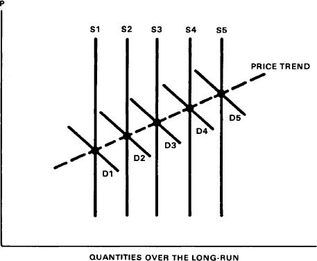
FIGURE 30:

LONG-RUN RISE IN PRICES.

How can the present inflation in the U.S. be analyzed in terms of Figure 30? Here, as in Figure 29, we show both D and S schedules shifting simultaneously in their historical directions and proportions. D is seen to be increasing at a faster rate than S—and exactly the same juxtaposition of events took place in postwar U.S. Details on why and how this inflationary process transpired, and the crucial role played by government expansion of the money supply would take us beyond the scope of this book. Suffice it to say that the following general proposition emerges: whenever the rate of increase in D exceeds the rate of increase in S, prices will be able to increase because the “excess demand” enables sellers to ask for and get higher prices.

Shortages Caused by Increased Demand

Before we end this chapter, we should note some possible exceptions to the preceding analysis. What will be true for the long run need not always be true for the short run. For example, it is possible that, at any given time, in a given situation, selling prices may not be increased when D increases faster than S. That is to say, sellers may decide for some peculiar reason not to take advantage of the excess demand situation and charge what the traffic will bear. This hesitancy of sellers to raise prices was noted in our chapter on elasticity of demand; we now can analyze it again in the present context.

Imagine the following scenario. It is the first full peace-time year of car production following the Korean War and the post-Korean recession of 1953-54. The auto industry had expanded output by the customary 10 percent. This proportion of increase in S was supposed to be sufficient to satisfy the expected average increase in demand of 10 percent, and would enable prices to remain stable. But the best-laid plans of the auto firms were upset by what actually took place. Whereas S was increased 10 percent, D increased some 30 percent as a result of wartime pent-up demand. Clearly, sales were running ahead of expectations. What effect did this excess demand have on selling prices at the retail level?

The first sign that D had increased relative to S was the acceleration in car sales at a rate faster than expected. It was apparent that producers had underestimated demand. There was little question that long before the end of the selling period the stock of cars on hand would have been sold out at the original selling prices, resulting in shortages. Plainly, dealers had a grand opportunity to immediately raise their prices, charge what the traffic would bear, and increase the profit margin per unit sold. What did they actually do?

Non-Price Rationing

Although selling tactics varied, dealers generally adhered to similar practices: they did not overtly increase their selling prices. How, then, did they ration the scarce cars among their scrambling customers? As follows: Those customers who did not want to wait in line for cars offered bribes to the dealers by paying above list-price, and dealers were disposed to accept. Thus, dealers did covertly what they feared to do openly: raise prices in line with the excess D and charge what the traffic would bear, bargaining with each customer.

In most cases, however, customers who did not want to pay the higher price in the form of a bribe paid it in another way: they waited in line on a first-come, first-served basis. Although queueing up on the dealer’s waiting list does not incur a monetary cost, it does involve a psychic cost—the cost of waiting for something that one wants to enjoy sooner rather than later. (This time-preference will be discussed in Chapter IX.)

Now for the main question: Why didn’t sellers, faced by an obvious excess-demand shortage, behave exactly as expected under the law of market price and raise their prices? One possible answer is: As noted on previous occasions, sellers may be fearful of the social taboo against charging what the traffic would bear. By not raising prices when it was economically feasible to do so, they were apparently currying the public’s favor, foregoing short-term monetary gains in favor of long-run goodwill.

Connected with this possibility may have been the dealers’ belief that the unexpected surge in D was abnormal, purely temporary—that next season’s sales would return to normal—so why bother to raise prices and alienate customers for a purely short-term gain? Thus, it is not unusual for firms to forego short-term profit opportunities in favor of possibly greater profit opportunities in the long run.

Price Controls and Precautionary Pricing

We have seen that social taboos against sellers charging what the traffic would bear may exert a deterrent effect on price increases during periods of increasing demand. Social forces can also work in the opposite direction: they may induce firms to increase prices sooner than otherwise. In the early 1970’s, government wage and price controls induced firms to abandon their policy of not raising prices until their costs had increased.

In the past there were fewer social taboos against firms raising prices in response to rising costs. This is why firms had, for a long time, avoided raising prices during periods of increasing demand until such time as their costs began to increase. In this way they could blame rising costs (not rising demand) for their price increases. Today it is a different story. Government wage-price controls—real or threatened—have introduced a new source of uncertainty—a stop/go tendency of first imposing controls, then relaxing and terminating them. During the 1970’s this induced firms to resort to precautionary price increases.

Reliance on precautionary price-raising can be explained by the excess-demand environment created by inflationary policies of government. These inflationary policies have consisted of vastly expanded Federal spending, on the one hand, and deficit financing by the Treasury and the Federal Reserve monetary authorities, on the other hand. As a result, total purchasing power in the economy had exploded at a faster rate than the supply of consumers’ goods. This inflationary environment is very hospitable to the raising of prices by firms—indeed, it is the prime factor that enables prices to rise in the first place.

When selling prices are eventually raised, and continue to rise as long as excess-demand conditions permit, government threatens to move in with wage-price controls. Since these controls freeze selling prices for an indefinite period, firms realize that it may be profitable to rush to raise their prices and beat the anticipated price freeze before it is too late. Thus, we have the bitter irony of government inflationary policies, on the one hand, and the expected wage-price controls, on the other hand, working in tandem to induce firms to raise prices sooner than otherwise.

Conclusion

It is market demand that ultimately determines prices. True, in practice it is the firm that establishes the selling prices and determines how much to supply the market. But in the final analysis, this is about all the firm can do; in all cases it ultimately has to reckon with the market. It is market demand that ultimately ratifies or vetoes the firm’s price and quantity decisions. Will the firm set P too high or too low? Will its Qs be too high or too low? Or will there be market-clearing? Only the market can tell.

Appendix WILL THE REAL SUPPLY STAND UP?

The point of this Appendix is simply this: the reader should be alerted to the fact that the treatment of the supply concept in this chapter is radically different from the usual treatment in other books. Thus, the reader should know that in contrast to this chapter, which treats supply as an ex-post concept, the Standard text treats supply mainly as an ex-ante concept.2 The distinction between ex-ante and ex-post was used in Chapter V to analyze the nature of decision-making and to state the maximizing principle. However, it also applies directly to the present analysis of the firm’s supply decisions concerning how much to produce and at what price to sell. Let us see how.

We have already seen that, in the case of supply, the ex-post concept is relevant only to the actual provision by the firm of goods for sale in the market. For this reason, ex-post supply is graphically depicted as a vertical line or curve, indicating that a given total quantity is being offered by firms at varied prices. It is, indeed, the only way to properly depict the actual supply situation in any given market, for any given type of product. Furthermore, for the purpose of graphically depicting the market, with its array of demand and supply sides, only the ex-post supply curve should be used to intersect the demand curve, as in Figure 20 above.

In stark contrast, the typical textbook depicts the market as an intersection of the familiar demand curve with an upward-sloping ex-ante supply curve (as shown in the following Figure B). The ex-ante supply curve looks essentially different (see the following Figure A) from the vertical ex-post supply curve for the simple reason that it is relevant only to the pre-production phase, when the firm is still contemplating or planning its production program, in preparing to decide: How many units should be produced? What price should be set?

In the ex-ante phase of its decision-making, the firm has not yet produced anything—it has not even launched any production and it surely has not yet put a single unit of its product for sale on the market. Thus, in the ex-ante state, there exists no such thing as a “supply” of any sort; at this point, “supply” is nothing more than a gleam in the firm’s eye; the firm is merely preparing to produce varying quantities, depending on which of various possible prices it thinks is likely to prevail.

FIGURE A:

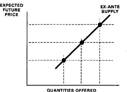
FIGURE B:

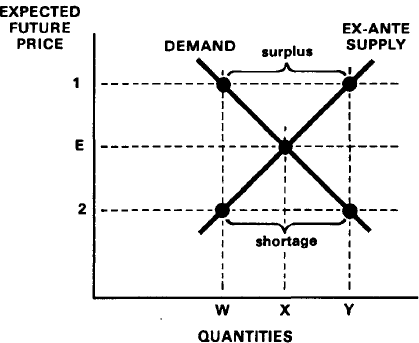
EX-ANTE DEMAND AND MARKET PRICE.

The mind set of the firm in the ex-ante planning stage is illustrated in Figure A. As a first approximation, it says: If firms expect prices to be higher tomorrow, they will be willing and able to produce more and, vice versa, if they expect prices to be lower, they will produce less.

The reasoning behind this upward-sloping ex-ante S involves considerations of costs and profit margins. With respect to costs, we will see in Chapter XI that higher rates of production (i.e., at higher rates of productive capacity) involve higher unit costs, whereas at somewhat lower rates of output unit costs are less. Thus, expectations of higher prices are supposed to induce firms to produce more, either because profit margins will be higher or, at least, the higher costs will be covered by the expected higher prices. Conversely, expectation of falling prices puts a damper on the firm’s plans: lower prices threaten expected profit margins, which can be preserved only by falling back to lower rates of production and lower unit costs.

So far, so good. We return now to the main point of this Appendix. My argument is not with the idea of the ex-ante S curve itself: it is a useful snapshot of how firms feel about producing varying quantities at various expected prices. Rather, what I find disturbing is the textbook tradition of using the ex-ante S curve for the purpose of describing the market process (as in Figure B), a procedure that contrasts sharply with use of the vertical ex-post S curve in this chapter (see Figure 20 above).

True, both of these figures are similar in being diagrams of demand-and-supply concepts; both have intersections of D and and S to indicate the market-clearing (equilibrium) price which the market will tend to reach; and, in both cases, surpluses will occur when prices are set too high, while shortages will emerge when prices are set too low. But there the similarities end. Whereas the vertical ex-post S curve of Figure 20 is a realistic, appropriate depiction of actual market supply, the ex-ante S curve is a pure phantom, having no real existence except in the ex-ante minds of those planning future quantities to be produced by the firm.

To be sure, textbooks find it useful to rely on diagrams like Figure B for the purpose of outlining the potential causes of surpluses and shortages, for which modest purpose such figures may be suitable. Thus, Figure B is able to show that surpluses would arise if ex-ante plans set prices and supply in excess of demand (at level 1) and that shortages would emerge if prices and supply are set too low (at level 2). In contrast, the vertical ex-post supply curve is not only more realistic and correct, but, no less significant, it also enables a more complete analysis, as already shown in this chapter.

It is in this latter respect that the ex-ante S curve suffers a serious and embarrassing lapse, specifically in attempting to analyze the case of a surplus. First, let us assume that firms set their prices too high (at level 1) and produce quantities Y; but at that high price the quantity demanded falls back to only quantity W, creating a surplus of WY. Then the argument goes, firms begin to slash prices to get rid of surpluses, and they also cut back on production until, at price E (equilibrium level) they produce only quantity X, and thereby are able to clear the market. However, what is usually overlooked by texts is the following curious lapse in analysis.

What is overlooked is the fact that, in order to dispose of the surplus WY, the firms must slash prices from level 1 all the way down to level 2 in order to clear the market of the quantity Y they had produced at the expected price (level 1). Thus, the market-clearing price in this case is at level 2, not level E as Figure B would have us believe! That is, price-level E could serve as a market-clearing price only if the firms had initially produced only quantity X to sell at price E; since they, instead, produced the larger quantity Y to sell at price-level 1, there is simply no way they can clear the market of the total quantity except by slashing prices all the way down to level 2.

In fact, if they had cut prices only down to level E, there would still remain some surplus—the amount XY! Clearly, there is no market-clearing here—not until prices are slashed to level 2. In this price-slashing binge firms would be gliding right past price E, precisely because it would not clear the market. Thus, in this first go-around there is no way the firms can discover the market-clearing price E—something which they would be able to discover in Figure 20 above, with its ex-post curve. To repeat, use of the ex-ante supply curve prevents realistic analysis of the market as a feedback mechanism and of the price adjustments firms must make to achieve market equilibrium.

 

____________

3This section is based on Hobe Morrison, “Scalpers Gyp Legit Talent,” Variety, Jan. 16, 1957, as reprinted in Paul A. Samuelson, Robert L. Bishop and John R. Coleman (eds.), Readings in Economics (3rd edition. New York: McGraw-Hill Book Co., 1958), pp. 184–188.

4A noteworthy exception is the treatment by Armen A. Alchian and William R. Allen in University Economics (3rd ed., Belmont, Calif.: Wadsworth Publishing Co., 1972), Chapter 6.

• 1See Thomas Sowell, Knowledge and Decisions (New York: Basic Books, Inc., 1980) for an elaborate analysis of how—despite the complex structures and environments of the modern division of labor—the free society and its market-price system generate, transmit, and apply “authentic” knowledge in the realms of economics, law, and politics. For an earlier treatment, see Friedrich A. Hayek, The Constitution of Liberty (Chicago: University of Chicago Press, 1960).
• 2Excellent examples of this type of supplementary work are John C. Goodman and Edwin G. Dolan, Economics of Public Policy: The Micro View (2nd ed., St. Paul: West Publishing Co., 1982), and Walter E. Williams, America: A Minority Viewpoint (Stanford: Hoover Institution Press, 1982).
• 3Add to this the obfuscations, deliberate or inadvertent, of those messianic types who would deliver us from all our travails by imposing their illusions, myths and Utopian visions on the rest of us—and it follows that the task of discerning and explaining the true nature of economic existence becomes so much more difficult,
• 4For the rest, for the purpose of greater illustration and application of analysis to public issues and policies, I defer for the most part to the numerous useful works devoted especially to this purpose. These works, including books of readings, provide ample supplementary materials that illustrate at length how economic theory or principles manifest themselves in practice and how economic analysis can be applied to practical problems.