Foundations of the Market Price System

CHAPTER IX PROFITS—AND OTHER INCOMES

This chapter is mostly about profits. Wages and other incomes are briefly touched upon, but the spotlight is on profits. The importance of profits should be clear: the firm which earns profits is also the prime generator of other incomes, including wages and salaries, as we saw in Chapter IV. In that chapter we also saw how profits can be increased by improved technology and cost reduction. In Chapter VIII we saw how changing market conditions affect selling prices and profits. In the upcoming Chapter X we will see how profits serve as the central motivating force of free-market firms. In the present chapter, our primary purpose is to explain the nature of profit itself—why the firm necessarily seeks profits and why profits are a justified return.

Controversy over profits—their justification and morality—has raged since the ancient and medieval taboos against the taking of interest on loans (“usury”). People did not understand why the moneylender should get back more than he lends. In modern times, Marxists and other socialists have maintained that profits are the result of “exploitation” of workers by capitalist owners of the means of production. For Marxists, profits belong to the workers in the first place, and are taken from workers only through capitalistic “monopoly” ownership of the means of production. Hence, for Marxists, profits are no more a deserved or earned income than is interest. In the following pages we will see why the taboos and attacks on profits are wide of the mark.

I. Introductory

First of all, production takes time. This fact is obvious, and may even seem trivial, but for economics the element of time is crucial. Why? Before we answer this question, we should briefly describe why production is not an instantaneous process but takes time to unfold and materialize.

Phases of the Production Process

As we have already seen, the entire production process involved at least three time phases. First comes the ex-ante phase during which the firm is engaged in estimating, speculating, planning, and investing activities—all centered around its decision as to what to produce, how much, and at what price. This is followed by the actual physical production phase. During this period, means of production are combined according to appropriate techniques that bring the product through stages of maturation until it is made ready for market. Finally comes the ex-post phase during which the product is supplied to the market, and the firm is able to see whether the sale of its product proceeds as planned.

Thus the entire production process embraces more than a physical-technical coordination of production resources in some appropriate technical combination. It includes also the ex-ante planning period and the ex-post or after-the-dust-has-settled period of reckoning. Even if physical production were somehow magically instantaneous, it still takes time to plan it (especially prices and quantities) and to assess results in the aftermath of market sales.

Moneylender vs. Entrepreneur

Overall, then, the production process involves not only the acquisition and use of means but also a prolonged waiting period until the product is completed, marketed, and hopefully sold. Seen from another viewpoint, when the firm undertakes production, it is making current outlays on factors of production in anticipation of future sales or payoff. To paraphrase a once popular commercial, the firm typically pays out now in order to fly later. In a general sense, therefore, the firm is essentially in the same position as the moneylender: both make a current outlay of money in exchange for a future payoff.

True, there is a technical difference between moneylending and entrepreneurial production by the firm. The moneylender makes his current outlay of money to the borrower in one lump sum, whereas the firm makes its current outlays mostly in the form of a series of regular payments to workers (wages), landlords (rent), power companies, and other resource, owners from whom it purchases or hires the necessary means of production. But this is merely a superficial technical or institutional difference, and does not alter the essential similarity between moneylending and production: both processes are inter-temporal in that they span a period of time from the present into the future. Furthermore, they are similar because the future payoff is characteristically expected to be greater than total current outlays. In the one case this increment is called interest; in the other it is profit.

To be sure, profits earned by firms consist of more than the equivalent of interest. As we will see, total profits earned by the firm include not only (a) a pure interest component but also (b) an entrepreneurial component due to uncertainty and risk, and (c) a purchasing-power component to compensate for changes in the value of money associated with changing price levels. Each of these components plays a vital role in determining the size of the firm’s price spread (profit margin) between the expected selling price and the unit costs incurred in production. Let us first examine the interest-rate component.

II. Time-Preference and Pure Interest

The first question we must ask is: What exactly is the connection between the interest rate earned in moneylending and the profit rate earned by the firm? The answer given by economics is straightforward: The common basis for both the interest rate and the profit rate is man’s natural time-preference. But what is “time preference”? Briefly, and somewhat crudely, it means that man prefers the present time to the future, other things being equal.

Meaning of Time-Preference

To be more precise, the time-preference axiom refers to the deeply-rooted and widely observed fact that, other things being equal, people prefer to enjoy any given satisfaction or good in the present rather than to enjoy the same good in the future. To put it another way: For any given goal set by a person, he would prefer to realize it sooner rather than later. The less the waiting time, the better. As one writer has put it, a bird in the hand is worth more than a bird in the bush. It makes no difference whether the goal is material or spiritual, tangible or intangible—man prefers to achieve his goals in the shortest possible time, ceteris paribus. Conversely, the more distant the future achievement of any given goal, the less valuable does the goal become. Man attaches a “disutility” to waiting: postponement of consumption involves sacrifice.

It is important to stress the sameness of the object of satisfaction whose present availability is preferred to its future availability. Unless it is the same satisfaction that is being time-compared, it would be possible to raise the following objection: In wintertime, why would anyone prefer ice delivered then to ice delivered in the following summer when the weather is very hot? The fallacy here is the assumption that summer ice is literally the same good or satisfaction as winter ice. To be sure, ice is ice when regarded purely in terms of its physical-material properties. But the fact that cooling ice-in-summer provides significantly greater, and hence different, satisfactions than ice-in-winter compels us to regard the two ices as different goods rather than the same good.

Life Is Not Forever

Why is time-preference so deeply rooted in the nature of man? Some writers explain it in terms of an obvious physiological fact: Man does not live forever. Alas, man is mortal! The life he enjoys must someday be ended. Nothing is more certain in life than death—unless it be taxes, to paraphrase Dorothy Parker.

Furthermore, although death may be as certain as taxes, uncertain is the duration of the life-span of any given person. The mortality tables have it all clearly laid out—the variability of individual life-spans. This only compounds the time-scarcity problem for the individual. How much time does one have left? How much time does one need to accomplish his goals? Is there time enough? If not, which time priorities are to be assigned to one’s goals? Can one tailor any given goal in order to fit the cloth of time available? Can one afford to postpone any given goal?

Time a Scarce Resource

As Böhm-Bawerk once put it: “[We] humans live out our lives in a temporal world . . . our Today, with its needs and cares, comes before our Tomorrow, and . . . our Day-After-Tomorrow may perhaps not be assured as at all.” There it is. Finite but indeterminate lifetime makes it even more uncertain that we can satisfy all our wants, regardless of other means available. So long as tomorrow is “not assured,” any satisfaction postponed today may never be realized.1

In this connection we can also invoke the maximizing principle (Chapter V) according to which man always acts in the expectation that his action will leave him better off than otherwise. This implies that, other things being equal, man will want to accomplish more rather than less within his given lifetime. Given man’s mortality, it becomes clear that time is the scarcest of means at man’s disposal. No matter how any given person manages his own time-scarcity, the fact remains that the only way to assure fulfillment of a given goal is to realize it sooner rather than later, ceteris paribus. Postponement of a goal only courts the likelihood it will never be fulfilled.

Time-Preference Axiomatic

Best of all, however, the validity of the time-preference theorem does not need to rest on psychology or physiology as above (e.g., the temporal limitations of human life, impatience, the disutility of waiting). As L. von Mises has put it, time preference is simply a “categorical requisite” of human action:

[E]ach individual in each of his actions is forced to choose between satisfaction in various periods of time. . . . The very act of gratifying a desire implies that gratification at the present instant is preferred to that at a later instant. He who consumes a nonperishable good instead of postponing consumption for an indefinite later moment thereby reveals a higher valuation of present satisfaction as compared with later satisfaction. . . . If he were not to prefer satisfaction in a nearer period of the future to that in a remoter period, he would never consume and so satisfy wants. . . . The knowledge provided by this insight . . . refers to every kind of want-satisfaction, not only to the satisfaction of the vital necessities of mere survival.2

Present Goods vs. Future Goods

At this juncture, we should introduce the important distinction between “present goods” and “future goods.” This distinction is based on the fact that any given good can be made available for consumption either in the “present” or the “future.” Present goods, then, are simply goods which are presently available for present consumption. This category embraces all consumers’ goods that are ready at hand for direct or immediate consumption, including leisure and money. Money, to be sure, is not directly consumable itself, but since it is readily exchangeable for consumers’ goods, it is a present good par excellence. For example, the money lent by the moneylender or paid out currently to workers and other resource-owners by the firm is classified as a present good.

In contrast to present goods are future goods. As the term suggests, these embrace all goods that only in the future can be regarded as present goods. Thus, this category includes future product—goods that will be completed only at a future date. It also includes goods-in-progress that are expected to emerge as consumers’ goods at some future date, as well as capital goods that enable production of consumers’ goods for consumption only in the future. They also include any claim on present goods in the future, such as money to be repaid by borrowers to moneylenders; hence, the promissory note (IOU) given by the borrower at the time of the loan is a future good. Similarly classified as future goods are securities such as stocks and bonds, which constitute claims to future income.

Inter-temporal Exchanges

We can now readily describe the activities of both the money-lender and the firm in terms of present goods and future goods: both are essentially engaged in exchanges of present goods for future goods. The moneylender typically exchanges a lump sum of money (present goods) for the borrower’s promissory note or IOU (future goods). Since the IOU promises repayment to the lender at a future date, it constitutes a future claim against the borrower. All loan transactions therefore are in essence an exchange of present goods (creditor’s money) for a future good (the debtor’s IOU).

Productive activities by the firm can be similarly described as involving essentially inter-temporal exchanges of present goods for future goods. The firm’s current outlays of money on wages, rent, materials, and utilities can be classified as present goods. These current outlays are made in exchange for an ownership claim or title to the future product turned out with the help of workers, landlord, suppliers, and utility companies. Thus, all employment transactions between firm and worker involve an exchange in which the firm makes a series of present payments to the workers in exchange for rightful title to the product. Furthermore, the firm’s outlays of money for factors of production also constitute an investment made in the present in expectation of profits at a future date (Chapter IV).

Premium vs. Discount

We can now restate the time-preference theorem in terms of present goods versus future goods. Man attaches a greater subjective value to present goods presently available to him than to the same goods available only in the future. For example, a person would rather hold a $100 bill now than hold it, say, five years from now, other things being the same—that is, disregarding the possible risk of not getting it back later from a borrower, and disregarding possible changes in the value of money due to a changing price level. Conversely, man attaches a lower subjective value to future goods, available only in the future, compared to the same goods available in the present. Thus, a moneylender who is promised a $100 bill in future repayment by a borrower (future goods) will now lend the borrower less than $100 (present goods) in exchange for the IOU of $100.

In effect, we have just described the difference between “premium” and “discount.” Even though these two terms are actually two sides of the same coin, there is a difference. Premium reflects the higher subjective value we attach to present goods that are presently available rather than in the future—the greater value attached to the convenience of earlier availability as compared to deferred availability. In the market place, present goods always command a premium or higher price over future goods.

In contrast, discount reflects the lower (“discounted”) subjective value that we attach to future goods because they suffer from deferred availability—they are characteristically available only after a period of waiting. That is to say, discounting reflects the sacrifice involved in postponing present consumption and in waiting for its future availability. Hence, the market attaches a lower price to future goods compared to present goods that are presently available.

A Loan Transaction

For example, assume A possesses a given stock of wealth, say, ten barrels of sugar. Along comes B and asks to borrow the 10 barrels for one year. To this A replies: Okay, but I request repayment of 11 barrels. B agrees, and it’s a deal—a deal that reflects a premium of one barrel of sugar, or 10 percent attached by A to the one-year loan. This case is one possibility. An alternative scenario could run as follows: B offers to repay A 10 barrels of sugar one year from now in return for 10 barrels borrowed today. But A protests, and suggests instead that he lend B only 9.1 barrels in exchange for the deferred repayment of 10 barrels. If B agrees, it’s a deal—in effect, the same kind of deal as above, except that it reflects the other side of the coin, the discount: 10 barrels available a year from now is today worth only 9.1 barrels to A, revealing a present discount rate of 0.9 barrels, or about 10 percent of the 9.1 barrels lent.

Thus, premium and discount turn out to be merely two sides of the same coin. These two different ways of expressing valuations always refer to the same goods or object. They differ only with respect to which end of the time-span of goods availability one happens to focus on—on whether the goods availability is present or future. The premium emphasizes the greater value attached to presently available goods, whereas the discount emphasizes the lower value attached to the same goods available only at a later date.

Firm Discounts the Future

Just as we can describe loan transactions in terms of “premium” and “discount,” so can we describe production and selling by the firm as involving a premium or a discount. As we saw in Chapter IV, the firm “works back from price” whenever it plans its current production. That is to say, it peers into the future to estimate its future market demand—its expected selling price and the quantities to be produced at that price. It then determines the profit rate it would like to earn on each unit to be sold (the unit profit rate). The residual obtained by subtracting the unit profit margin from the unit selling price represents the self-imposed limit on how much the firm can profitably spend currently on factors of production for each unit of output. Now, where does the premium or discount element enter into these calculations?

Let us assume a firm that is making product X and expects to sell it at some future date—say, a year from now, for $100. At this price it expects to sell its entire future output of X, which is currently in the works. Thus, there is a time-spread between current factor outlays and future selling of its product. The firm will have to wait until some future date before it can sell its output and reap the harvest of its current outlays on production. For the firm, therefore, the future selling price of $100 constitutes a future good. Like any future good, which is naturally handicapped by its deferred availability, this potential future $100 for each unit sold will have a lower present value compared to the same $100 were they presently available. That is to say, the future $100 is translated into a present discounted value.

The rate at which the future $100 is discounted is, of course, a subjective matter, depending on the subjective valuations of the firm’s executives. For instance, if the firm is willing to expend only $90 now on factors of production on each unit produced, in exchange for the future $100, the $10 difference represents the rate of discount. Conversely, the future $100 price represents a $10 premium attached to the current total outlay of $90.

Pure Interest Rate

This brings us to a crucial point. Implicit in the concepts of “premium” and “discount” is the pure interest rate, which is actually the subjective time-preference rate. Hence, the “pure” interest rate should not be confused with the actual market or “loan” rate of interest, of which the pure rate is but one component. The other two components of the market rate allow for (a) uncertainty and risk factors attached to the loan, and for (b) changes in the purchasing power of the dollar. (More on this in Section III.) Thus, the actual rate of interest paid on loans in the market comprises all three components: subjective time-preference, uncertainty and risk, and changes in the value of money. In our present discussion we will focus on the time-preference or “pure” rate of interest, unless otherwise specified.

In our sugar-loan illustration, the premium rate of 10 percent actually represents a pure interest rate; so does the discount rate. Both of these rates also reflect Mr. A’s subjective time-preference rate at the time of the loan. For example, if A had felt otherwise, and either (a) had asked a premium of 1.5 barrels for the 10 loaned, or (b) offered only 8.7 barrels in return for repayment of 10 barrels, both of these cases would have reflected a 15 percent rate of time preference: in the first case this rate is reflected in the 1.5 barrel premium, and in the second case the rate is reflected by the discount of 1.3 barrels. In both events the time-preference rate is the same 15 percent, which is also A’s interest rate.

We can now also see why the pure interest or time-preference rate can be described as the intertemporal exchange rate between (a) present goods presently available and (b) future goods available only at a later date. In our sugar illustration the 10 percent premium rate of interest was derived from the ratio of 11/10, while the 10 percent discount rate of interest was obtained from the ratio 10/9.1.

The “Price of Money”

The reader should not be misled by the customary notion that interest rates are related only to money loans. We have just seen, in our sugar illustration, that a loan transaction between creditor and debtor can take the form of non-money goods. Indeed, history tells us that as far back as the Babylonian King Hammurabi, more than 2,000 years B.C., people were making loans in non-money commodities. The only difference between a sugar loan and a money loan is that the former is transacted in barrel units of sugar, whereas the latter involves units of money (e.g., dollars).

For this reason it is also misleading to define the interest rate merely as the price of money, rather than in the basic universal terms of time - preference. First of all, interest-bearing loans can be made in non-money goods as well as money units, as we have just noted. True, in the modern economy, interest is usually paid in the form of money, but this does not make interest a purely monetary phenomenon. Indeed, at heart, interest is a reflection of universal time-preference.

For another thing, the word “price” is literally misused. A money “price” represents the full number of money-units asked by the seller in exchange for a unit of his goods. In contrast, an interest payment is only a fractional payment, only a part of the total sum of money-units being exchanged. For example, an interest payment of $10 on a loan of $100 is only part of the total value of the transaction.

Furthermore, the present “price” of $100 is simply another batch of 100 dollar-bills—no more, no less. That is to say, anyone who wants to “buy” some money can go to the bank and buy, say a $100 bill by paying with a check or 100 dollar-bills, the “price” of money here being simply $1 for $1.

Additionally, and more precisely, the “price” of any good—say, X, be it money or a non-money good—is equal to the amount of other goods that this good X can be exchanged for in the market. For example, if the market price of X is $5, it means that one unit of X is exchangeable for five dollar-units. (The “exchange rate” is 1:5.) On the other hand, from the point of view of one dollar bill, the “price” of that dollar is how much it can be exchanged for in terms of X (which is one-fifth of X). For this reason, the “price” of a dollar is not the interest rate but rather how much the dollar can be exchanged for in terms of the full array of alternative goods. Technically speaking, it is approximately the inverse or reciprocal of the general “price level” of all non-money goods. Thus, the higher the price level, the lower the “price of money,” and vice versa.

Saving and Investing

Finally, and most fundamentally, the “price of money” concept mistakenly implies that the natural phenomenon of the interest rate arises only in loan transactions between parties A and B. This misconception gives rise to the expression that interest is “the price of a loan,” which implies that a loan necessarily involves two separate parties, the lender and the borrower. However, a person can “lend to himself” as well as to others. For example, individual savers or groups of savers can “borrow” their own accumulated savings and invest these savings, without resorting to loans from other parties. Indeed, the classical concept of the “capitalist-entrepreneur,” who was a central figure in spearheading the Industrial Revolution, was based on this notion of the saver and capital accumulator investing his own wealth without recourse to borrowing from others.

In all such cases, where people indicate a relatively lower time-preference by saving and investing in productive ventures—whether their own or others’—the presumption is that the saver-investor believes his investment in production will yield him a future consumption that will be greater than otherwise. This does not mean that savers-investors value the future absolutely over the present, but merely that they prefer a future consumption that would be greater than otherwise. In working to make for themselves a “better future” than otherwise, they in effect hasten the realization of their future.

Interest-Rate Tables

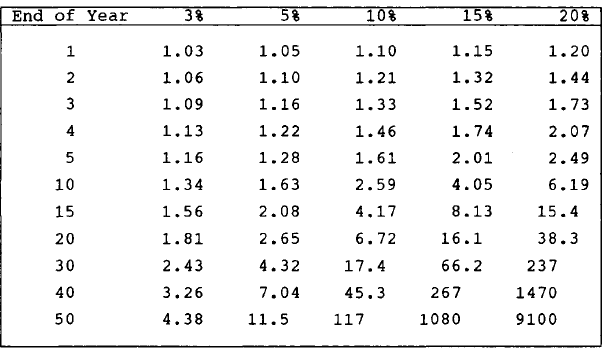
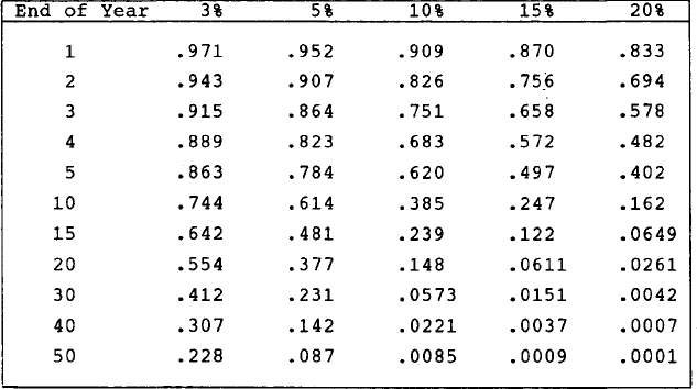
We have now seen that inter-temporal exchange transactions can involve money and non-money goods, and can also involve an investment of one’s own accumulated savings rather than a loan transaction. We should also note that loans can be made for consumption purposes (consumer loans) as well as for production purposes (commercial loans). In any case, the various possible rates of exchange between present goods and future goods—that is, the various rates of subjective time preference as well as premium and discount—can be numerically expressed in the form of interest tables, such as Tables III and IV, which are condensed versions.

For example. Table III can illustrate the terms of a premium-type loan transaction. Imagine a current loan of $1,000 to be repaid in 5 years at 15 percent interest per annum. Table III tells us that the premium rate attached to each dollar borrowed is 2.01 (see the first column for the year 5, then across to the 15 percent column). We then multiply 2.01 by $1,000 and get $2,010. This is the total to be repaid by the borrower: it consists of $1,000 principal plus $1,010 premium interest.

TABLE III

Compound Interest on One Dollar

In contrast, we can use Table IV to illustrate the terms of a discount interest loan. Imagine a borrower who offers to repay the lender $1,000 at 15 percent interest, at the end of 5 years. Table IV tells us that the rate at which the future $1,000 should be discounted by the lender is .497 (see the first column for year 5, and then across to the 15 percent column). We then multiply .497 by $1,000 and get $497. Hence, in a 15 percent loan, $497 is the present discounted value of $1,000 to be repaid 5 years from now; that is, the lender who wants to receive $1,000 in a 5-year, 15-percent loan should lend out no more than $497.

TABLE IV

Present Discounted Value of a Future Dollar

Some Propositions

While we have these two interest tables at hand, we should examine them for several important propositions implied in their numerical structure. The first implied proposition should be familiar by now: the greater is the time-preference rate, the greater is the numerical rate of interest, or the lower is the present discounted value. This can be seen by scanning each year-line from left to right. In Table III, for example, the numbers increase in value to reflect the higher time-preference or interest rates. Similarly, Table IV tells us, as we scan from left to right, that lower and lower present discounted values apply to the increasing rates of time-preference or interest.

We now come to a second proposition implied in these interest tables: the longer the time-span involved in the inter-temporal transaction, the greater is the premium rate of interst, or the lower is the present discounted value. This can be seen by scanning each percent column from the top down. In Table III, for example, the numbers increase in value, reflecting the greater premium attached to transactions of longer duration. In Table IV they drop in value, reflecting the increased rates of discount applied to such transactions

A third proposition implied in our tables runs as follows: the time-preference or interest rate is always positive, never zero or negative. In other words, inter-temporal exchanges will always be transacted at a premium or discount rate of interest. For instance, A will never lend B 100 units of X now for only 100 units or less to be repaid at a later date, other things being equal. This assumes A’s time-preference rate is the only determining factor in the terms of exchange, excluding personal considerations such a friendship or blood relationship with B.

Time-Preference: Relative vs. Absolute

In this connection it is important to note that positive time-preference is relative, not absolute. An absolute time preference means that a person provides only for present consumption or acquires only present goods, and never saves any current income for future consumption (those “rainy days”) nor acquires any future goods (such as IOU’s or securities).

Such absolute time-preference is conceivable only under two unlikely conditions. One would be a catastrophe-ridden world, where everything was going to “come to an end” at any moment, and there would truly be “no tomorrow.” With catastrophe hanging overhead like a Damocles’ sword, no one could be blamed for living it up today, with nary a care for the morrow. The other condition would be a non-scarcity world of absolute abundance, like the Garden of Eden. Here everyone could truly be a pure consumer (a pure non-saver), never having to worry about saving something for future consumption.

At the opposite extreme is the case of absolutely no time preference. This means that people have no desire to live “in the present”—to do any consuming now—but prefer to save everything for the future. At this extreme rate of abstinence, the human species clearly could not survive; it would simply perish!—which makes this condition totally unrealistic. Furthermore, if people literally never consume anything. including the things they might buy with their savings, there is obviously no point in doing any saving in the first place.

However, there are people who have relatively low time-preference rates and, therefore, tend to be savers as well as consumers. That is to say, even while they consume significant portions of their current income, they also set aside significant amounts for future consumption by saving for those rainy days, retirement, or other future goals. Savers characteristically have longer time horizons than non-savers: for them the future stretches over a greater span of years than for non-savers; the latter care more about “living it up” today, care less about future consumption. Yet, even among savers, the rate of saving will vary according to one’s age, circumstances, and preferences.

Time-Preference: High and Low

Clearly, then, real-world rates of time-preference must lie mostly between the one extreme of absolute time preference and the other extreme of absolutely no time preference. Real people are characterized by relative rates of time-preference, ranging from relatively “high” to relatively “low” time-preference rates, and varying from individual to individual and from age to age. That is to say, even though people prefer to consume now rather than later—other things being the same—they do save some of their income and allocate it toward future consumption. By saving varying proportions of their income, they divert varying amounts of current consumption toward future consumption.

People with relatively high time preference tend to use most or practically all of their income for present consumption, and save very little, if anything. Indeed, some people may consume more than their current income (“live beyond one’s means,” so to speak) either by living off their accumulated savings, or by borrowing the savings of others whose time-preference rate is lower and who, therefore, save more.

On the other hand, people with relatively low time preference tend to postpone present consumption at a greater rate than people with high time preference. They are the people who defer much consumption by saving significant parts of their current income. These are the savings that are usually channelled into investment —via the financial system (e.g., the stock and bond markets)—in the growth of productive capacity of firms. Firms depend on these savings to supplement their own internal saving or cash flow, and invest them in new capital goods (see Chapter IV).

Because investment by firms in capital goods tends to increase productivity and reduce unit costs of production, thereby increasing profits, savers are reasonably induced to share in these profits by investing in firms. Thus, people are always tending to balance their time-preference and the disutility of postponed consumption against the advantages of investing in the higher productivity of expanded capital structure. Hence, it is the saver-investor, possessed of relatively lower time preference, who provides the capital for ever more elaborate (“longer”) processes of production which, in turn, increase the productivity and standard of living of the community. In other words, the saver-investor provides the present goods that enable the firm to produce future goods, in return for which he acquires a claim to a share of the profits.

Calculation of Profits and Costs

We can now see how Table IV, on present discounted values, can help illustrate the profit calculations of the firm. Since the firm is a discounter of future values—seeking to keep its present costs below its expected future selling price—Table IV becomes the relevant table. On the one hand, this table deals with present discount factors, while on the other hand, the firm must necessarily attach a discounted value to its current factor outlays—a value calculated on the basis of its expected future selling price.

Assume, for example, that the firm is producing a computer to sell at $100,000 a unit, each of which takes two years to produce. The firm wants to earn a 15 percent profit as its pure interest rate. Working back from its future price of $100,000, the firm knows it must limit its unit costs to something less than $100,000. The question now is: What is this cost-ceiling that will allow the firm to earn 15 percent pure interest over two years on each unit produced?

If we were, instead, involved in a loan transaction, the calculation would be fairly simple. A two-year loan at 15 percent, repayable in the sum of $100,000, would call for a present cash outlay by the lender of only $75,600 (obtained by multiplying the discount factor .756 by $100,000). That is to say, $75,600 represents the present discounted value of $100,000 repayable at the end of two years. The firm, too, like the moneylender, makes a present discounted payment in exchange for a greater payoff in the future. But there the resemblance ends. For practical reasons, the firm does not make its present discounted outlay to workers and other owners of production-factors in one lump sum as does the moneylender. In practice, the firm breaks its total outlays down into a series of regular weekly or monthly income payments, which enable wage-earners, rent receivers and materials suppliers to make their own current expenditures for consumption and production purposes.

Discounting Current Factor Outlays

Thus, the difference between making a series of current payments to factor-owners, stretching over two years, as compared to a mere lump-sum loan of cash, introduces an insignificant complication in the calculation of present discounted values of current cash outlays. Whereas the lender makes only one lump-sum outlay at the start of the two-year period, and then waits a full two years for repayment of every dollar of principal, it is otherwise with the firm.

The firm does not have to wait a full two years for a payoff on each of its currently paid-out dollars to factor-owners. Indeed, the first month’s outlays wait 23 months for their payoff; the second month’s outlays wait 22 months for their payoff; the third month’s outlays wait 21 months; and so on, until the final monthly outlay waits no longer.

Over the two-year period as a whole, therefore, each of the firm’s current monthly outlays to factor-owners involves not one present discount factor (e.g., 0.756) but rather a series of them, each numerically lower than the preceding one. Theoretically this implies that each month’s outlays would have to be determined by use of lower and lower discount factors, and therefore payments to workers and others would be larger each successive month. In practice, however, it is more convenient for both the firms and factor-owners to have the payments made in uniform, unchanged amounts. How can this practical institutional complication be handled?

Making Regular Payments

Since the firm will be making twenty-four identical monthly outlays, the firm can calculate an approximate present discount factor by using the twelfth or mid-point month as its guide. In Table IV we see that the discount factor for the end of the twelfth month, at 15 percent interest, is 0.870. This implies that the average of all monthly discount factors is 0.870, and that the sum of the different present discounted values will total about $87,000 over the two-year period. That is to say, the firm must limit its current outlays to $87,000 per unit produced, yielding a profit margin of $13,000 for each unit sold at $100,000.

In practice, of course, there is no assurance that the firm will be able to hire or purchase factors of production at market prices (wage rates, rents, etc.) that will be low enough—that is, low enough to keep unit costs from exceeding the $87,000 limit which the firm will be willing to spend for each unit produced. The firm’s inducement to employ labor and other resources depends crucially on the current market price of the resources. Thus, if one or more of the resources needed is overpriced, the firm may have to cancel the venture altogether—unless it finds a way to economize on some inputs, or decides to accept a reduced profit margin.

Relevant Costs of Production

This brings us to a vital consideration: Which costs should the firm include in its calculation of the cost of production? First of all, costs can be calculated either as a marginal cost (MC) or as a per unit or average cost (AC). The MC is simply the total cost that will be involved in producing a given quantity or batch of products. The AC is simply the total cost (or MC) divided by the number of units to be produced, yielding a per-unit cost. Now, to return to our question: Which types of costs should be included in the calculation of MC or AC?

It helps to realize, at the start, that not all expenditures by the firm are to be regarded as relevant costs—costs that will necessarily be incurred by the forthcoming production. For example, as we will see below, not every dollar expended for plant and equipment is a relevant cost. Furthermore, relevant costs must be broken down into (a) explicit costs, and (b) implicit costs. Leading examples of each category are as follows:

Typical explicit costs include:

Wages and salaries,

Rent,

Interest,

Materials,

Power,

Repairs and maintenance.

In contrast, implicit costs include such items as:

Depreciation of plant and equipment,

Implicit wages and salaries of owner,

Implicit rent on owners land and factory facilities.

What is the real difference between explicit and implicit costs? Explicit costs, usually referred to as “out of pocket” expenditures, always involve an outlay of money for goods and services purchased or hired for the given production program. They can be measured strictly on the basis of the purchase price of the given factor. Also, these factors are usually “short-lived” and therefore “expire” in the process of production: the factor is either technically transformed (e.g., materials) or is “embodied” in the product (e.g., labor, power). They are readily measurable or calculable. Implicit costs, in contrast, usually involve one or another complication when it comes to their calculation.

Implicit Earnings

For instance, in cases where the owner of the firm provides professional services (managerial, legal, etc.) so that the firm does not have to hire these services on the market, resources are being used even though no specific money expenditures are involved. Thus costs of production are incurred which are equivalent to the wages and salaries that the owner could have earned by selling his services to other firms. These foregone earnings constitute an opportunity cost whose value is imputed from the market value of the owner’s services to his own firm.

Similar reasoning applies to the use of land and factory facilities that are owned by the firm but which are used in production instead of being rented to the market. Here the rent that could have been earned by selling these resources directly to the market are definitely an opportunity cost. Therefore their use in production by the firm involves a cost of production whose value is imputed from the rent that could have been earned on the market.

Depreciation and Interest

Why is depreciation of plant and equipment placed under implicit costs rather than explicit costs? Does not the acquisition of equipment, for instance, involve an outlay of money and, therefore, should be treated as an explicit cost? Well, equipment usage is complicated by the fact that it is durable or “long-lived,” and therefore does not get used up (“consumed”) in a single act of production. This has two important implications. First, the value of the equipment used up in a single act of production is usually only a fraction of the total purchase price. Second, at any given moment, equipment commands a resale value—either as productive equipment that still is useful, or as mere scrap. How does this help us calculate the economic cost of using equipment in production?

From the above it should be clear that the cost of equipment used in production—and the same goes for the physical plant—is measured not by its original purchase price but only by the portion of it that is actually used in the current production program. This portion is measured by the difference between the equipment’s current resale value (at the start of the current production period) and its prospective resale value (at the termination of the production period). This difference in resale values is called depreciation, and reflects the economic cost of the wear-and-tear of the equipment used in production.

A final note about interest costs listed among explicit costs above. On loans received by the firm, only the interest portion of the obligation—not the principal—is included as an explicit cost. Inclusion of the principal would involve double-counting, since the proceeds of loans typically become embodied in explicit expenditure items such as wages and salaries, materials, etc.

Specifically, the funds could have been invested in stocks and bonds, and could have earned dividends and interest for their owners. When owners of the firm invest in production instead of stocks and bonds, they are foregoing an opportunity to earn income elsewhere. The interest and dividends they could have earned on the financial markets they now want to exceed by investing in production instead—for earnings that are expected in the form of profits.

Profits as Opportunity Costs

We have now completed the first, and main, leg in our journey to uncover the nature of the profit margin. It is time, also, to briefly survey our results. Our first goal has been to link the basic component of the profit margin to the pure interest (time-preference) rate. Both moneylender and firm are engaged in the inter-temporal exchange of present goods for future goods. Since the present value of future goods is typically discounted, both moneylender and firm naturally attach a discount to their future payoffs. Here lies the reason for both the interest on money loans and the profit margin earned by firms.

We can now also see why the profit margin reflects an opportunity cost—the equivalent of what the firm could have earned elsewhere, by investing in financial assets instead of in production. Owners of the firm always have the option of investing their savings in the purchase of securities that yield interest or dividends and capital gains. By investing, instead, in production, they expect to earn at least the equivalent of what they could earn in the foregone investment opportunities. In effect, the owners of firms are merely lending their capital funds to themselves instead of to others. Furthermore, it makes no difference if the firm, in addition to investing its owners’ savings, also borrows the savings of others via the financial markets: in both cases it will want to earn at least the equivalent of alternative earning possibilities.

III. Uncertainty and Inflation

We said at the start that the profit margin consists not only of a time-preference or pure interest component, but also of “entrepreneurial” and “purchasing power” components. The entrepreneurial component is included because of the hazards and risks faced by the firm due to the uncertainty of selling successfully in the market. The purchasing-power component is included because of changes in the value of money that are related to changes in the money supply and general price level.

Uncertainty and Changing PPM

If we were living in an imaginary world devoid of any uncertainty and risk, and in which the purchasing power of money (“PPM” hereafter) was perfectly stable, the profit margin could then consist only of pure interest. In the real world, however, there are no riskless markets or stable PPM.

Instead, there is constant uncertainty of market demand and selling conditions, and the PPM is subject to depreciation due to government monetary inflation and rising price levels. Both market uncertainty and changes in PPM affect ex-ante planning and ex-post sales experience in unpredictable ways and, therefore, compel the firm to provide against adverse effects by appropriate provision for both entrepreneurial and PPM components in the planned profit margin.

Impact of Uncertain Demand

How does market uncertainty influence the firm’s ex-ante planning of its profit margin? In our preceding illustration we had the firm earning a $13,000 profit on each unit sold at $100,000, representing a 15 percent return on a two-year production project. But this assumed certainty of sales—that the firm would actually sell every unit produced (say, 200 units) at the expected selling price of $100,000. Such certainty of sales is possible only in the unreal world of static, unchanging market conditions in which the firm has complete knowledge of market demand and exactly how many units to produce.

However, unchanging market conditions do not exist in the real world, where demand and supply are in constant dynamic flux and market-clearing prices become unpredictable. In a world of market uncertainty and unpredictability, ex-post realized sales may or may not turn out as planned in the ex-ante. How does this uncertainty prospect affect ex-ante profit planning?

Impact of Reduced Sales

Suppose, for instance, that the firm wants to hedge against the possibility that it will not sell all of its 200 units, in which case it would have to slash its price in order to sell out the remaining unsold units. Such a prospect would, of course, also reduce the expected profit rate of $13,000 per unit. In order to minimize the effects of these adverse prospects on profits, the firm can, say, add a five percent margin for uncertainty and thereby enlarge its ex-ante planned profit rate from 15 to 20 percent. In principle, this increase in profit rate can be sought in two ways: (a) by lowering the ceiling on its unit costs from $87,000 to $83,000 (discount factor 0.833 multiplied by $100,000), or (b) by raising its expected selling price to about $103,700. Or it could plan a combination of (a) and (b). Its final choice will, of course, depend on whether it can effectively reduce its unit costs or whether, in its judgment, the market demand is inelastic against a price increase. In any case, the greater the uncertainty and risk attached to a given project, the larger will be the entrepreneurial component of the ex-ante profit margin.

If market demand is seriously disappointing, quantities sold will be less than expected, selling prices will have to be slashed, and profits will be less than expected. The drop in profits may either be slight or so great as to wipe out the profit margin or even prevent the firm from recouping some of its factor outlays.

Impact of Excess Demand

Of course, the market could throw a pleasant surprise by having demand exceed the firm’s expectations. For example, assume demand increases at the same time that product is being released to the market, resulting in an excess demand for the product. As we saw in Chapter VIII, the firm might be able to spot this incipient shortage fairly early in the selling period, and decide to raise its price to take advantage of the unanticipated bulge in demand for its product. If so, its ex-post profit margin would surely exceed its ex-ante planned margin due to the emergence of entrepreneurial profit.

Thus, we see that the entrepreneurial profit component enters into the picture only after the firm makes due allowance for pure interest or time - preference. It can emerge both in the ex-ante planning phase and in the ex-post selling phase. In view of inevitable and pervasive market uncertainty, the entrepreneurial component must be regarded as a categorical element of the firm’s profit margin. But whereas the pure-interest component is always positive, the entrepreneurial component can be either positive or negative.

Impact of Inflation

Finally, the firm’s profit margin must make due allowance for prospective changes in the purchasing power of money (PPM), especially in periods of rising or falling prices. Since we are living in an “age of inflation” marked by rising prices and shrinking PPM, it is reasonable for the firm to anticipate a decline in PPM by the time its product is selling on the market. Rising prices and declining PPM, in turn, mean that the dollar buys less and less as time goes by. Failure to allow for this inflation effect in the profit margin will, other things being equal, yield profits whose real purchasing power is less than planned.

In order to minimize the inflation impact on the purchasing power of its ex-post profits, the firm will include an inflation component in its ex-ante profit margin. The size of this PPM component will vary, of course, with the anticipated rate of inflation: the higher the rate of price inflation anticipated, the larger will be the inflation component, and the larger will be the ex-ante profit margin. So long as inflation is anticipated, the firm will hedge against it by inflating its profit margin.

But this can be a hazardous game. There is no guarantee that the anticipated market demand will increase sufficiently to absorb the inflated profit margin. As we saw in Chapter VIII, increases in selling prices can be realized only when market demand is increasing faster than market supply. If for any reason such buoyant demand is checked, or even slowed down, the roof can cave in; market demand will resist the inflated selling prices and the firm will fail to realize anticipated sales.

Market Rates of Interest

At this point we should note that market rates of interest charged in the loan market will tend to reflect entrepreneurial risk and PPM considerations as well as pure interest rates. Thus, market rates of interest will tend to increase not only when subjective time - preference increases, but also when investments become riskier and when price-inflation intensifies. For this reason the loan-market rate of interest will tend to reflect gross profit margins in the economy.

IV. The Tail That Wags the Dog

In a sense, the preceding is merely prelude. In the present section we draw a variety of implications of both economic and general significance that follow from the preceding sections. Human action in the “economic” spheres of production and exchange is merely a particular expression of principles of human action in general. We have already argued this with respect to the maximizing principle and self-interest. We now argue similarly with respect to the implications of the preceding discussion of time - preference and profit planning.

Futurity of Human Action

A moment’s reflection should make us realize how extensively man’s goals and actions—be they centered on consumption or production—apply to the future, near or remote. We have seen again and again that the firm’s production decisions are always made in the present with an eye to the future. But this principle applies as well to virtually the entire realm of human decisions, not only to economic affairs. Other things being equal, the only difference among goals is how far each one reaches into the future. Many goals pertain to the very near future, while others are posted in the remote future. By contrast to the future, the present permits man time to do but two things: (a) make choices of future goals, and (b) apply means for the accomplishment of those goals.

Economics as such cannot tell us anything about the making of ex-ante choices, except that they are individual or subjective and that, except where man has full knowledge of the data related to his decisions, choices cannot be made with certainty of outcome in a world universally subject to changing conditions and uncertainty. Thus, economists as such are no more qualified than anyone else to advise people on what decisions to make in their personal or business affairs. However, with respect to the application of means for the achieving of goals or ends, economics is qualified to assert certain principles of universal relevance.

Imputation Process: Ends and Means

The first significant implication is the existence of an imputation process, a general process by which value is ascribed from one source to another. More precisely, the imputation process describes how means or resources acquire value from the value attached to the product they help produce or the goals they help realize. As a general principle, people value the means at their disposal strictly according to the value they attach to the given end which the means can achieve.

In the case of the firm, the discounted present value attached to current outlays on factors of production is an example of an “imputed” value—a value derived from a prime source, the expected future selling price of the product to be produced by labor and other factors. For example, the value of a bricklayer’s labor (e.g., his hourly wage rate) is imputed from the value of the building he helps build. Similarly, the value of machinery in a factory depends on the value of the steel or automobiles it helps produce. As a general principle, the greater the value attached to a future product or other goal, the greater the value that can be imputed to the means employed in achieving the given end.

Capital Value

This helps us understand the technical concept of capital value. “Capital values” are involved whenever you hear questions like these: What is the value of a given piece of land? What is the value of a given building that consists of office-space or residential apartments? What is the value of a given piece of machinery? In each case, the general answer is the same: The value of these capital goods depends on the value of the product or service they can help produce. Thus, land that is sitting on major oil deposits will be valued more than land suitable only for cattle-grazing. Machinery that is useful for producing automobiles will be valued more than machinery useful only for making motorcycles. In the case of buildings, let us imagine the following case.

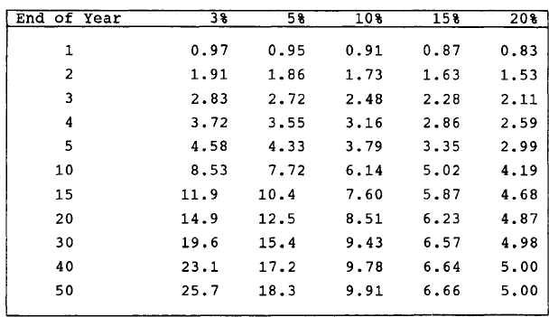
Assume an office building has been put up for sale. What price can its owner expect to get for it? What price should the potential buyer be willing to pay for it? In both cases. Table V can help. Basically, we need to know the following: (a) the physical durability of the building, specifically the years of “life” left in it; (b) the estimated total rent (income) expected from occupants of the building during the remaining lifetime of the building; and (c) the rate of profit the buyer seeks to earn on the funds invested in the building. For illustrative purposes let us assume that (a) is 20 years, (b) is $40 million, and (c) is 10 percent. (Let us also assume there are no risk and PPM elements involved in the deal.) Given this basic information, the following Table V helps us derive the capital value of the building, which then can serve as the price to be negotiated between seller and buyer.

TABLE V

Present Discounted Value of a One-Dollar Annuity

An Illustration

In consulting Table V, we locate the desired information by scanning across the 20-year line until we spot the factor 8.51 in the 10 percent column. This factor is a present discounted value, compounded annually. It tells us that it is worth paying $8.51 today for an annuity that promises to pay one dollar annually for the next 20 years, that is, a total income of $20, stretched out evenly over 20 years (i.e., $1 each year, hence called “annuity”).

How do we apply this tabular information to our problem? Since the estimated expected total income is $40 million, and assuming this income will be evenly distributed over the 20-year period, we therefore have an investment that promises to yield $2 million a year (equivalent to 2 million one-dollar annuities). By multiplying the factor of 8.51 and 2 million, we arrive at a capital value of $17,020,000. This means that an investment today of $17,020,000 (a) would yield a 10 percent return when taken in the form of $2 million a year over 20 years, totalling $40 million, and (b) $17,020,000 is the top price the buyer should offer for the building. Of course, less should be offered if there is any risk attached to the investment.

A Definition

We can now define capital value without too much difficulty: it is the present discounted value imputed to a stock of productive assets or factors that is expected to yield its owner a stream of earnings over a given future period. The concept applies to any durable good whose future earnings can be estimated. It also applies to securities, such as stock, which represent shares of ownership in the capital assets of a firm, and, hence, are a claim to a share of its earnings (i.e., profits) in the form of dividends.

Capital Losses, Capital Gains

What would happen to capital values if estimates of future earnings of the asset increased or decreased? This question is very relevant in a dynamic real world of perpetual flux in prices and earnings. This brings us to the twin concepts of “capital gains” and “capital losses.” Suppose that, in the case of our 20-year building, while negotiations for sale/purchase are underway, the earnings prospects suddenly drop because of the construction of new competitive buildings in the same neighborhood? Say, instead of the expected $40 million, prospective income is revised downward to only $32 million.

Given the same desired 10 percent rate of return, we now apply the 8.51 factor to 1.6 million (i.e., $32 million divided by 20 years) and come up with a capital value that has, to no one’s surprise, dropped to $13,616,000. This drop in capital value from $17,020,000 to $13,616,000 constitutes a capital loss for the owner of the building. He would now have to shave the price of his building in order to induce someone to buy it.

Just as a drop in prospective earnings results in a lower capital value or capital loss, so does a rise in prospective earnings mean a capital gain. Thus, if there is an increased demand for office space that appears long-lasting, and earnings prospects increase to $50 million, say, this would bring a rise in capital value to $21,275,000 and enable the owner to ask for a higher price on the market.

Share Prices and Wealth Effects

The stock market is notorious for its daily fluctuations in the earnings prospects of traded shares of common stock. For this reason, the daily quotations of share prices undergo echoing changes. When the earnings prospects of Company X spurt upward—due to a very promising new product, say—you can expect an immediate upward surge in the market price of its shares. And vice versa, if this company’s earnings face a downturn, you can expect a dip in its share price. Once again, prospective future values determine current values.

Furthermore, capital losses and gains also signify corresponding changes in one’s wealth status. Even when one is not actually buying or selling productive assets or securities, it is possible to undergo a change in wealth status; so long as one owns such assets, he is vulnerable to fluctuations in their capital value.

To go one step further, an increase in the capital value and wealth of any firm represents, in effect, an increase in its profit rate as well. And vice versa, an increase in its profit rate brings with it an increase in capital value and wealth. The three change in related fashion. In any case, such are the hazards of the market: constant change in prospective earnings, and related changes in capital values and wealth, place a premium on being able to read the uncertain future.

Imputation and MR vs. MC

Although our illustrations of the imputation process have come mostly from economics and business, imputation processes apply in a general way to all human action. In making choices and in applying means toward achieving given ends, future value always determines present value; that is, the value attached to one’s goal, purpose, or object of future enjoyment determines the present (albeit discounted) value of the means that can be applied toward achieving the given end.

In our present context, a corollary implication runs as follows: man will apply means toward the satisfaction of a goal only when the value attached to the goal exceeds or at least equals the value attached to the means of achieving that goal, depending on how distant in time is the goal. Colloquially put, man will put out effort so long as the eventual payoff seems worthwhile, or the benefit exceeds the cost. Or, conversely, man acts because the goal is sufficiently worthwhile to warrant the cost.

In the language of economics, man will act on a goal only when its marginal revenue (MR)—that is, the total amount of gain or benefit expected from the goal—promises to exceed or at least equal the marginal cost (MC)—that is, the total costs involved in achieving that goal. Since MC represents current outlays, it is calculated as a present discounted value. Therefore, the more distant the goal, the more must MR exceed MC. Also, in the case of the firm, since MR and MC consist of “batches” or “lumps” of dollars, these dollar totals must be divided by the number of units produced in order to yield a unit profit margin comparable to the concept of unit profits hitherto used.

Derived Demand for Factors

Another fairly obvious implication is that the firm’s demand for factors of production (labor, etc.) is a derived demand—derived from the anticipated demand for its product. As we saw in Chapter II (Figure 4), the firm is essentially a go-between between people as demanders of products (consumers) and people as owners of resources (workers, etc.). In this intermediary role the firm relies on its estimate of future market demand as a guide to its current demand for labor and other resources.

In the case of consumers’ goods, the demand for factors is derived from the anticipated consumers’ demand; in the case of producers’ or capital goods, the demand for factors is derived from other firms’ demand for capital goods. In both cases, the firm will not hire or buy services, supplies, or equipment before it has estimated the market demand for its product. These estimates of market demand can be optimistic, pessimistic, or merely moderate, but in all cases the firm can be either right or wrong, due to market uncertainty.

The significance of this is that anticipated market demand emerges as the ultimate determinant not only of the quantity and selling price of the firm’s product but also of the quantity of resources the firm uses and the factor prices (wage rates, rent, etc.) it pays to resource owners. The quantity of resources used, multiplied by the prices paid to resource owners, constitutes the total cost of production as well as the income earned by resource owners. The total cost divided by the number of units produced yields the unit or average cost (AC). It is this AC which represents the present discounted value that the firm derives when it “works back from price,” to determine the profitable limit to costs.

“Cost-of-Production” Theory of Price

A still further significant implication of the imputation principle is that it undermines the cost-of-production theory of price. This popular concept was given authority by classical economists of the early 19th century, and was converted into the “labor theory of value” by Marxists for partisan purposes. In response to the traditional question in economics, “What determines price?”, this theory has alleged that it is the cost of production that determines selling price. In effect, it is a “cost-plus” theory of pricing.

With a bit of simplification, the cost theory runs as follows: First, the firm calculates its cost of production per unit of output; it then adds on a profit margin, and voila!, it arrives at the market selling price. In the Marxist version, all costs boil down to but one: labor effort expended by workers. Labor alone creates the “value” of products that is the basis of their “exchange-value” in the market place. Thus market price is supposed to reflect the number of man-hours of labor embodied in the product.

Marxist vs. Non-Marxist Versions

Marxist proponents of the labor-value theory of price claim that the firm’s profits represent “exploitation” because their source is the “value” created by workers. On the other hand, non-Marxist proponents of the cost-theory of price allege that firms in the market economy can earn profits at will. For them, profits are merely an addendum to the costs of production, and their size is determined entirely at the discretion of the firm.

More precisely, firms are alleged to have the power to “administer” prices—to raise prices whenever they wish to increase profit margins. This power to “administer” prices is also the core of the “cost-push” theory of price inflation, which holds that firms cause inflation merely by raising prices. The fallacy of the “administered price” concept will be discussed in Chapter XI. Here it suffices to assert that, in the real world, firms in no way possess the magical power to increase profit margins at will merely by raising prices.

Market Determines Prices

The general cost-of-production theory of price runs smack against the theory of price presented in this book. As we have maintained all along, it is the market, with its forces of demand and supply—and not the firm—that is the ultimate determinant of selling prices. In Chapters X and XI we will see even more forcefully that it is not of ultimate importance that in practice it is firms who post selling prices. No firm can regard its posted price as the ultimate selling price—the price at which the demander actually decides to buy. The final selling price is entirely up to the state of market demand and supply. And, after all, it is this final market price that really matters; the initial price posted by the firm in the ex-ante phase is, by the nature of the case, no more than a tentative price, subject to final validation by the marketplace. In no way can the firm be consoled by its ability to post a price that straightaway must face the market test.

“Working Back from Price”

Furthermore, we have seen in the present chapter that far from costs determining prices—as is commonly assumed—it is just the reverse: market price determines costs! Before the firm can profitably decide how much to spend on labor, materials, rent and other costs, it must estimate the price at which it can sell its product. Only after the firm has made its best estimate of the future price can it then profitably work back from price—that is, subtract its unit profit margin from the price and determine the limit to its current outlays or AC.

This is not the place to get bogged down in the doctrinal history of the controversy over the cost-of-production theory of price and the Marxist labor theory of value. It suffices to note that the cost theory was massively challenged by economists of the late 19th century such as W. Jevons, C. Menger, and E. von Böhm-Bawerk. By 1913, P. H. Wicksteed could confidently assert the victory of the “marginalist” revolution against the cost-of-production theory as follows: “[T]he idea that cost of production already incurred determines exchange value [i.e., price] turns out to be a reversal of the true relation. It is the anticipated value in exchange [i.e., expected selling price] that determines what cost of production the producer will be willing to encounter. . . .” (underlining and brackets mine).3

Labor’s Claim to Product

Let us discuss some further drawbacks of the Marxist “labor” theory of price. After this will come a critique of the more general “cost” theory of price.

First of all, in the modern division of labor there is no way that workers can legitimately claim the full market value of the product. The reason is simple: labor is not the only resource used in production. Alongside workers are landlords, moneylenders, materials suppliers, and equipment owners, among others. As it is, workers account for the bulk (more than 70 percent) of the national income; the remaining 30 percent goes to several other groups. Unincorporated business—e.g., self-employed professionals, farmers—gets about 10 percent, while earners of profits, rent, and interest account for the other 2 0 percent.

There is an even more important reason that labor cannot lay claim to the full product. On the basis of what we said in Section II, in the case of our computer firm, it is clear that the final product—the 200 computers—belongs to the firm and not the workers. This is based on the nature of the exchange embodied in the employment contract: the workers agree to offer 40 hours, say, of labor in exchange for $5 per hour wages. That is to say, their only claim on the firm is $5 for each hour worked. Therefore, since the product is owned by the firm, the full proceeds from their sale on the market, including the profits, belong to the firm and not the workers. Hence, there can be no “exploitation” in the sense of taking from the workers what belongs to the workers.

True Source of Profits

Furthermore, the true source of the profits themselves is the market demand for computers; more precisely, the expenditures made by final customers. It is physically impossible for the firm to earn profits from any other source except the customers in the market who like the computer enough to buy it. In no way can workers be the source of profits when it is entirely up to the market to yield them. That is, the product must sell out in the market place before the firm can earn profits as expected.

Imagine, for example, what would happen to profits if planned sales of the computer fail to materialize. Indeed, let us assume the worst of all possible outcomes: not one unit is sold—the firm loses out in competition with a rival’s cheaper, superior model. In this extreme case, we get an interesting result: workers and other resource-owners have already gotten their $87,000 income (in wages, rent, etc.) from the firm’s previous outlays for each unit produced—but the firm, alas, gets no profits at all!

It should be evident, therefore, that it is not the workers’ labor that is the source of profits but the market demand. Indeed, since the market determines whether there are profits, and how much, it is the market that also determines whether there is “exploitation” in the Marxist sense!

For example, assume that our computer firm sold all 200 units at $13,000 profit for each unit after resource-owners had earned their $87,000 (with workers getting $60,000, say) for each unit produced. The emergence of profits makes this a case of “exploitation” in the Marxist sense. But if, on the other hand, none of the computers was sold, yielding zero profits to the firm, we would have to conclude that the same $60,000 received by workers for each unit produced was not an “exploitation” wage after all! We thus arrive at the curious conclusion that the deciding factor as to whether there is “exploitation” is the market! That is to say, it is the customers who, every time they like a product and buy it, thereby validate the firm’s profit expectations and thereby cause the workers to be “exploited”!

“Labor” Unit a Fiction

This brings us to the critical point: There is no such thing as a standard unit of “labor value” in the first place. There is no such entity that is supposedly produced by the worker. There are only man-hours of labor expended on the product, the wage-rate for which—in a market economy—depends ultimately on the market demand for the product. The best way to see why the “labor value” unit is a fiction is to visualize the following case.

Imagine a self-employed worker who has no “boss” to “exploit” him, but who makes his living by producing and selling leather shoes for barter-exchange with others in the market. He works some 60 hours a week, say, and produces 10 pairs per week. Thus, each pair of shoes takes six hours of labor. On the market, he seeks to sell the shoes in exchange for sugar, candles, oils, and other consumers’ goods.

Theoretically, in order to give his labor a uniform market value over time, our shoe craftsman should seek in exchange the same amount of other goods for each pair of shoes. That is to say, he should seek the same “price” for each hour of labor expended on his shoes. For example, he expects that one pair will always fetch ten pounds of sugar, or one gallon of oil, or three dozen candles, and so on. But in practice, this expectation is rarely fulfilled. Sometimes he gets more sugar, oil, or candles for a pair of shoes, sometimes less. In effect, the “purchasing” power of his shoes—that is, of hours of his labor—is not stable but fluctuates from day to day.

Labor’s Fluctuating Value

What is it that causes this fluctuation in the “value” of our shoemaker’s hour of labor? How is it possible for the product of an hour of labor to fluctuate in its exchange-rate with an hour’s product of another worker?

Let us first rule out changes in the quality of product; we assume the quality is uniform over time. Given this uniformity of quality in product, the shoemaker reasonably expects the same, constant exchange rate between his pair of shoes and other goods. Let us also rule out changes in the shoemaker’s subjective valuation of his shoes, which might induce him to sell them at higher or lower exchange-rates because of a higher or lower subjective value attached to his shoes compared with other goods.

We will also rule out any changes in productivity or “efficiency”—in the number of shoes produced per man-hour. We assume productivity is constant: one pair produced every six hours. For example, if his productivity somehow increases—say, to one pair every five hours—his total weekly output also increases and he can offer more pairs for each unit of other goods “purchased” in the market. Thus, his increased supply would compel him to reduce the “price” of his shoes. Conversely, if his productivity declines, and he produces only one pair every ten hours, each hour of his labor now exchanges for less of other goods. It is as though he had raised the “price” of his shoes relative to that of other goods. All this we assume away.

Role of Market Demand and Supply

There remains only one possible answer as to why his hour of labor fluctuates in exchange-rate with other goods: fluctuations in market conditions of demand and supply. And we do not mean changing conditions in the shoe market alone, but in all other goods markets as well. As we saw in the preceding chapter, shifting demand and supply conditions bring on changes in price. It makes no difference whether it is a barter economy or a money economy: shifting D and S conditions will cause changes in exchange-values or “price relationships” between one good and another.

For example, in a monetary economy, the changes in “price” occur in the changed exchange-rates between units of money and units of other goods—for example, the exchange-rate or price of beer can go from one can for 20 cents to one can for 30 cents. Similarly, in the barter economy, the exchange-rate or price commanded by a pair of shoes can go from one pair for one gallon of oil to one pair for a half-gallon of oil.

Thus, the market emerges as the primary cause of changes in the exchange-value of an hour of labor and, hence, is the ultimate determinant of the market value of a labor hour. And, as far as the market is concerned, it makes no difference whether the worker is “his own boss” or works for a firm; it is the market that determines the “price” commanded by any given product and, indirectly, determines the value attached to labor (or any other factor input) as well as the size of the profit rate.

Workers’ Control of Firms

Otherwise, in the free-market economy—which will be further analyzed in detail in the next chapter—workers are totally free to abandon their role of alleged “wage-slaves” and themselves undertake the entrepreneurial role of the firm. This they can do by organizing their own firm under so-called workers’ control; they can pool their savings, or borrow the savings of others through the financial institutions, and invest these savings in their own firm. But even so, they would themselves then have to make current outlays for wages and other factor payments, and to wait until their product is completed and sold before they could recoup their expenditures and earn profits for themselves.

Since, in fact, workers do not generally rush to buy out existing firms or establish new ones themselves—in order to specialize as entrepreneurs themselves—we can conclude that they prefer the existing division of labor between themselves as “workers” and others as “firms.” Whereas the firm must wait for its returns (profits), the worker gets his payoff now, without waiting. He prefers to take his money and run, as the saying goes. Thus, those who have relatively high time preference will tend to be attracted to the role of the “worker,” whereas those with relatively low time preference will tend to be the savers and “capitalists” who invest their own wealth in production. That is, the latter look upon their investment in firms as the means of achieving a future consumption that is greater than if they had not saved and invested.

Costs Are “Prices”

Now, as for the general cost theory of price, it too is heir to all the objections levelled against the Marxist labor-theory of value. In addition, it is embarrassed by an economic truth: costs are themselves “prices.” A wage-rate for labor is a price; so is rent a price; materials costs, too, resolve themselves into prices. And in every case these factor prices are determined by the same market forces of demand and supply that determine consumers’ goods prices. Thus, it is circular reasoning to argue that factor costs explain market price when these costs are themselves determined by the very same market forces they are supposed to explain in the first place!

Market Determines Wage-Rates

The dependence of factor prices and costs on market demand and supply can be exemplified by the wage-rate—the price paid for labor. In Figure 31 we see how the hourly wage-rate would be determined by market D and S.

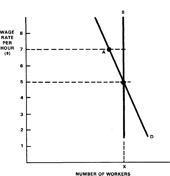
FIGURE 31:

MARKET DETERMINATION OF WAGE-RATE.

To simplify the exposition, let us assume a 40-hour work week. The demand schedule relates to the firms; it reflects their demand for workers—the number of jobs they would offer at various wage-rates. It possesses the characteristic slope downward from left to right, which means that, other things being equal, more workers would be employed only at lower wage-rates, and fewer workers would be employed at higher rates of pay.

On the other hand, the supply schedule relates to the workers: its verticality indicates that, at the given moment, there is a fixed number of workers who are seeking to work a 40-hour work week. But each worker has his own minimum “reservation price”—the minimum wage-rate below which he will not accept work. Thus, the hourly wage-rates acceptable to workers run from as low as $1.50 on up.

Cause of “Unemployment”

How does the market determine the wage-rate in a given field? Figure 31 says that any worker seeking a job can find one if he limits his wage demand to $5 an hour or less. The $5 rate would exactly clear the market: at this wage, the number of workers seeking jobs (X) is just equal to the number of jobs being offered (X). But at any higher wage-rate, say $7, workers would be inviting some unemployment: while the number of workers seeking jobs remains X, the number of workers being sought by firms has dropped to A, causing unemployment for AX workers. Clearly, at $7 the workers would be overpricing themselves, and as we saw in Chapter VIII, overpricing leads to unsold surplus which, in the case of workers, means “unemployment.” Unemployment is the market’s way of penalizing the overpricing of labor—the way it limits wage demands made by workers.

At first glance, it is the demander—the individual firm—which decides the highest wage-rate it is willing to pay, a limit it establishes as a result of “working back” from the expected selling price of its product. All firms together, therefore, comprise the market demand for labor. But, since firms are merely intermediaries between consumers and resource-owners, they come to realize sooner or later that it is the consumer who ultimately determines the limit to the wage-rate payable to workers.

Factor Costs Are Opportunity Costs

The cost-theory of price is mired in circular reasoning for another reason. The “costs” of producing a given good X are essentially opportunity costs: they reflect foregone opportunities, i.e., the other things that the given resources could produce if they were not used in producing X. Where technology permits, resources are generally useful in the production of a variety of goods. Labor, indeed, is the most nonspecific resource of all, since it can be applied in producing an infinite variety of goods and services. In lesser degrees, the same is true for land, materials, and many types of equipment. They are all more or less capable of serving diverse production purposes. For this reason, their utilization in producing any given good necessarily involves an opportunity cost. Indeed, the “opportunity cost” concept is made relevant precisely because of the diverse or non-specific uses to which resources can be applied.

Furthermore, the opportunity cost itself is measurable in terms of the earnings which the firm—or the resource-owners themselves—could have earned from using their resources in alternative uses. The market enables us to place a market value (“price”) on the alternative goods and services that could have been rendered with the given resources. Hence, for the firm, the “costs” of producing X merely reflect the potential profits from foregone opportunities to produce and sell other things. For the resource-owner, the “cost” of offering his resource to the producer of X reflects the earnings he could have received in some alternative production program.

To be more precise, the firm will employ resources for producing X only when it expects to earn more this way than using the resources to produce Y, Z, etc. Similarly, the resource-owner will offer his goods or services to the firm producing X only when he can receive more from this firm than he can receive from producers of Y, Z, etc. Thus, a producer of motorcycles will stick to producing them rather than motorized bicycles so long as—other things being equal—earnings from the former exceed potential earnings from the latter. Similarly, a design engineer will stick to his job at General Motors rather than switch to Ford so long as—other things being equal—his salary at GM exceeds the salary offered by Ford.

What Determines Opportunity Costs?

Although the concept of “opportunity cost” is valid as far as it goes, it nevertheless prompts us to ask: Doesn’t this concept itself beg the question? Indeed, there are several additional questions that beg for answers.

First, what determines the value of the given resources in their alternative, foregone uses? For example, if the value of resources used in making motorcycles is related to their value in making motorized bikes, it is proper to ask: What, then, determines their value in making motor bikes? This raises a second question: Why is the producer of X induced to use the given resources in making X rather than in making Y, Z, etc. Also, a third question: What induces General Motors to pay its design engineer a higher salary than he can get at Ford?

To the first question, the answer could very well be as follows: The present discounted value of resources used in making motor bikes is, as we have seen above, determined by the market price that demanders are willing to pay. Essentially the same answer pertains to the second question: The market demand and price for product X are presumably more attractive than in the case of product Y, Z, etc. An additional answer could be this: The firm is more efficient—is able to achieve lower unit costs—in making X than in making other products. This increased efficiency enables it to earn a higher profit margin. Both of these answers are also relevant to the third question: Either the greater demand and price for GM automobiles enables GM to pay its design engineer a higher salary than can Ford, or GM’s greater efficiency and profit margin enable it to do so.

Conclusion

What could have been a relatively narrow discussion of profits has turned into an economic Odyssey through the world of time and time—preference, pure interest, risk, and inflation—to say nothing of imputation processes, capital values, opportunity costs and the labor theory of value. From the simple concept of “production takes time” we went a long way to show that present values mirror future values. But this is in the nature of things. It is the “tail” of the future that wags the “dog” of today; tomorrow’s expected benefits induce or warrant the incurring of today’s costs. The “future” and “today,” it turns out, are linked inextricably in terms of benefit and cost.

 

____________

4Eugen von Boehm-Bawerk, Capital and Interest (South Holland, Ill.: Libertarian Press, 1959), Vol. I, p. 266.

5Ludwig von Mises, Human Action (New Haven: Yale University Press, 1949), pp. 480–485.

6Philip H. Wicksteed, “The Scope and Method of Political Economy in the Light of the ‘Marginal’ Theory of Distribution” (1913), reprinted in R. L. Smyth (ed.). Essays In Economic Method (New York: McGraw-Hill Book Co., 1963), p. 249.

• 1See Thomas Sowell, Knowledge and Decisions (New York: Basic Books, Inc., 1980) for an elaborate analysis of how—despite the complex structures and environments of the modern division of labor—the free society and its market-price system generate, transmit, and apply “authentic” knowledge in the realms of economics, law, and politics. For an earlier treatment, see Friedrich A. Hayek, The Constitution of Liberty (Chicago: University of Chicago Press, 1960).
• 2Excellent examples of this type of supplementary work are John C. Goodman and Edwin G. Dolan, Economics of Public Policy: The Micro View (2nd ed., St. Paul: West Publishing Co., 1982), and Walter E. Williams, America: A Minority Viewpoint (Stanford: Hoover Institution Press, 1982).
• 3A notable exception is the above-mentioned text by Goodman and Dolan which analyzes public issues in terms of moral, political and economic criteria.
• 4Add to this the obfuscations, deliberate or inadvertent, of those messianic types who would deliver us from all our travails by imposing their illusions, myths and Utopian visions on the rest of us—and it follows that the task of discerning and explaining the true nature of economic existence becomes so much more difficult,
• 5For the rest, for the purpose of greater illustration and application of analysis to public issues and policies, I defer for the most part to the numerous useful works devoted especially to this purpose. These works, including books of readings, provide ample supplementary materials that illustrate at length how economic theory or principles manifest themselves in practice and how economic analysis can be applied to practical problems.
• 6Before proceeding to the chapter-by-chapter introductions, it is necessary to point out that economic tracts—mainly because of materialist bias—usually omit the very important moral dimension, a dimension that is nevertheless relevant to economic reality—to economics in practice. First of all, economics as a social science is fundamentally concerned with exchange—“interpersonal transactions.” Exchange is inherent in every production and trade activity. Thus, the market-price system may be regarded as comprising multitudinous exchange transactions. Since exchange also infuses every interpersonal transaction in society at large, it also constitutes the basic coordinating mechanism of that most complex network of interrelationships called “society.”