Foundations of the Market Price System

CHAPTER VII PRICE-ELASTICITY OF MARKET DEMAND

After all is said and done, the law of demand is not enough. The reason: demand schedules come in a variety of slopes or price-elasticity—which makes all the difference in the world for the firm. Hence this chapter.

In the preceding chapter we visually alluded to the concept of price-elasticity of demand (Figure 9) by showing how market demand schedules, even though they all slope downwards from left to right, will in practice vary in their degree of slope or elasticity. We also noted that, technically speaking, demand schedules fall into three categories: elastic, inelastic, and unitary. In the present chapter we will not only explain the meaning of these categorical terms but will also show their extreme practical importance for the firm, as well as the special factors—social, technical, and economic—that help determine the category into which a given demand schedule would be expected to fall.

I. The Anatomy of Demand-Elasticity

The concept of elasticity of demand reflects the fact that, while the quantities demanded (Qd) by buyers are affected by the price of the product—as under the law of demand—the degree of responsiveness of buyers to a change in the price may vary from product to product, from person to person, and from time to time. That is to say, while a lower (higher) price set by sellers will be expected to increase (decrease) the Qd by buyers, the sensitivity of response of buyers to the given change in price will vary in degree. These different degrees of sensitivity or elasticity in Qd, in response to a given change in price by the seller, necessarily make the elasticity concept of greatest practical importance to the seller.

The Law of Demand Is Not Enough

The best way to get into the concept of price-elasticity of demand—“elasticity,” for short—is to realize that it is directly related to a situation often faced by the firm: the firm seeks to increase its total dollar sales receipts (hereinafter noted simply as TR for total receipts) by means of a change in its selling price, that is, by cutting it or raising it. Thus, in its quest for increased TR, the firm wants to determine the following: should it reduce its price, or increase it?

At first glance, this would seem a fairly simple decision: in order to increase TR, the firm should try to sell more units of its product. To accomplish this, the firm should reduce its price, according to the law of demand (see Chapter VI). So the decision seems obvious: cut the price. Right? No—wrong! It does not follow that selling more units at a lower price will necessarily increase the TR as well. True, the lower price will enable the firm to sell more units—according to the law of demand—but it does not necessarily follow that the quantity demanded (Qd) will increase sufficiently to offset the dollar loss due to the lower price received for each unit sold. It all depends on the elasticity of demand. Clearly, in such a pricing decision, the law of demand is not enough as far as the firm is concerned. So, without further ado, let us pursue this matter of elasticity.

How To Increase Total Receipts

Imagine a firm that wants to increase its TR because, say, it is confronted by a union demand for wage increases. Other things being equal, a wage increase would cause an increase in the firm’s total dollar costs (hereafter referred to simply as TC). Such an increase in TC, unaccompanied by a proportionate increase in TR, would in itself reduce the profit margin between TR and TC. (Note: total profits = TR - TC.) Now, one of the things the firm could try to do to offset the profit squeeze is to increase its TR sufficiently to cover the increase in TC.

Of course, the firm could try two other things in order to offset the wage increase and restore its former profit margin. Instead of increasing its TR, the firm could try to reduce its TC. On the one hand, the firm could lay off some workers and reduce its total wage bill enough to keep the TC at its former level. Or, it could install more efficient methods of production; this, too, would enable the firm to reduce its TC sufficiently to restore its former profit margin. In the present case, however, we assume that instead of reducing its TC, the firm seeks to increase its TR by selling a larger quantity of its product.

Quantity Demanded vs. Total Receipts

Now, according to the law of demand (Chapter VI), the firm would have to reduce its price in order to increase the quantity-demand (Qd) of its product. Since the law of demand is a matter of common knowledge, we would expect the firm to do the obvious and cut its price (P) in order to sell the larger quantity (Q) of its product. So far, so good—or so it would seem. But, as we have been intimating, the law of demand is not enough—not as long as the lower P fails to increase the Qd enough to offset the cut in price required to induce the increased Qd.

Let us illustrate graphically the problem of demand-elasticity now facing the firm. Figure 11 reveals a firm that has been selling 10,000 units at a price of $8 (see the dot 0). If the firm now decides to reduce the price to $5 in order to sell more units, it has no way of forecasting precisely how much the Qd will increase. This much, however, it does know: it would like the Qd to increase enough to offset the drop in P of $3 per unit sold; that is, it would like the TR to increase despite the lower price received. Only after it has actually cut its price will the firm be able to determine whether its TR has increased, that is, whether the Qd is sufficiently “elastic” to offset the price cut.

Selling More But Enjoying It Less

If after the price cut from $8 to $5 the Qd increases from the current 10,000 units to 24,000 units (see dot E in Figure 11), it is visually apparent that the response in Qd was comparatively great. More important, simple calculation reveals that the TR increases from the previous total of $80,000 (derived from P = $8 multiplied by Qd = 10,000) to a total of $120,000 (derived from $5 times 24,000 units)—despite the cut in P of $3 per unit! That is to say, the Qd proved to be sufficiently responsive to the price cut, and therefore able to offset the drastic price cut. Whether or not the increase of $40,000 in TR is actually enough to satisfy the firm’s goal, the fact remains that such a sensitive response in Qd is technically referred to as elastic. Elastic responses are precisely what the doctor should order if ever the firm has to cut its price, for only in such cases would the TR be expected to increase despite the price cut.

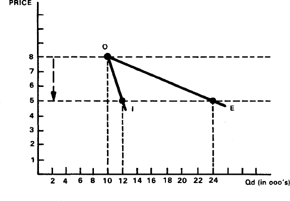
FIGURE

11: ELASTICITY OF DEMAND IN THE CASE OF A PRICE-CUT.

Things could have worked out just the reverse! If the Qd, instead of increasing to 24,000 units, increased only slightly—to only 12,000 units, say—the TR would show a decrease from its previous $80,000 to $60,000! (This is the result of the lower P of $5 times the 12,000 units sold, shown by dot I in Figure 11). Clearly the increase in Qd here is relatively small compared to the sizable price cut—it does not increase sufficiently to offset the hefty price cut—so that on balance, the TR decreased from its former level. The relatively insensitive response in Qd, indicated by the demand segment 01, is technically referred to as an inelastic response. Inelastic responses are precisely what the firm does not want to encounter if it ever has to cut its price, for in all such cases the TR would decrease in spite of the increase in Qd. This amounts to selling more but enjoying it less, so to speak.

The Unknown Demand Schedule

At this point we should note some additional properties of the demand schedule that are practically important to the firm. First of all, only after the firm changes its selling price can it get some idea of the slope of demand for its product. More precisely, at best it could discover no more than the segment of the demand that lies in the range of prices around its current price (e.g., the segments 01 and OE in Figure 11). Indeed, so long as the firm continues to sell a given quantity at a given (unchanged) price—e.g., 10,000 units at $8, in Figure 11—the only thing it really knows about the demand schedule is a single “dot”—the dot 0 in Figure 11, which represents the current selling P of $8 and the Qd of 10,000 units. Only by a trial-and-error process of changing its P can the firm discover the slope of the demand segment nearest to its previous position or “dot.”

The second noteworthy thing is that the slopes of the demand segment in Figure 11 are basically different: the inelastic segment 01 slopes more to the vertical, while the elastic OE segment slopes more to the horizontal. And this is generally the case: whenever the demand schedule assumes a relatively vertical posture, it is technically identified as “inelastic,” whereas the demand schedule that slopes toward the horizontal is identified as “elastic.”

Elastic, Inelastic and Unitary

Omitted from Figure 11 is the oddball in-between case where the degree of elasticity is technically categorized as unitary—neither elastic nor inelastic. This is the extremely peculiar case where the TR remains the same as before—TR neither increases nor decreases—even though both the price and Qd have changed. In the case of a price cut, as shown in Figure 11, the unitary case would be represented by an increase in Qd to 16,000 units, which at $5 a piece yields a TR of $80,000, precisely the same amount as the original TR. Such a result can occur only in the very unlikely event that the Qd responds just enough to compensate for or offset the extent of the price change, as a consequence of which the TR remains virtually the same as before.

Third, it should be noted that the demand schedule (D), which consists of an array of possible “dots”—each of which represents a given P and the Qd at that price—for that very reason also consists of an array of potential TR’s which can be calculated from the respective P’s and Q’s. In other words, the D schedule may also be interpreted as a TR schedule. As the firm moves from one selling price to another, it encounters not only a change in Qd but also a change in TR.

Elasticity of Demand and Uncertainty

This brings us to the fourth and probably most important aspect of the demand schedule—at least as far as the firm is concerned: the TR does not necessarily change in the same direction as does the Qd under the law of demand. That is to say, under the law of demand it is always true that a significant price decrease will cause Qd to increase, but it does not necessarily follow that TR will also increase. (Similarly, a significant price increase will cause Qd to decrease, but it will not necessarily cause TR to drop, too. More on this below.) It all depends on the slope, or degree of elasticity of demand. As we saw in Figure 11, in the case of a price cut, TR will actually decrease when the D schedule is inelastic, even though the Qd is increased. Only when the D schedule is elastic will a price cut increase TR as well as increase Qd.

The direct implication of this possible discrepancy between changes in Qd and changes in TR is the uncertainty that it causes for the firm whenever it wants to change its price and increase its TR. Will a price cut, for example, increase its TR or decrease it? The same question, we will see, applies to a price increase. The firm cannot know for certain which of the two TR outcomes will occur unless it knows the degree of elasticity of demand—that is, unless it knows whether the D for its product is “elastic” or “inelastic” in response to a price change. How can the firm acquire such practical knowledge of the elasticity of D for its product? Before we answer this question, we must resume our graphic analysis of elasticity to include the case of a price increase.

A Note on Statistical Procedures

Before proceeding, we should note the technical problem posed by the fact that the raw sales data showing the TR change cannot be accepted at face value. The reason: in practice, some part of the TR change may be due not only to the given price change (e.g., the price cut) but also to changes in non-price determinants, such as tastes or income. As we saw in Chapter VI, the law of demand abstracts from the impact of the various non-price influences on Qd. In the present chapter, for the purpose of illustrating the elasticity concept, we are similarly abstracting from possible non-price influences on TR, in order to be able to focus only on the relation between price changes and TR changes.

As a consequence of this technical problem, posed by the complex nature of the raw TR data, a variety of statistical procedures have been required to enable, at least approximately, the elimination of possible non-price influences on TR and the calculation of an “adjusted” TR figure which is related purely to price. A similar statistical chore is required in order to compute the coefficient of elasticity, which is the traditional method of explaining the concept of demand-elasticity (see Appendix to this chapter).

The Hazards of Price-Raising

Virtually everything we have said concerning the case of a price cut applies with equal force to the case of a price increase. Assume, now, that our firm has tried the price cut as a means of increasing its TR and discovered to its dismay that market demand was inelastic, so that its TR was now lower than before! The firm, being guided purely by the law of demand, might believe that its salvation lies only in a price cut—not a price increase—reasoning that only an increase in Qd could bring the desired increase in TR. Let us assume, however, that in sheer desperation it tries the price increase route to its goal.

In Figure 12, our firm has decided to raise its price from $8 to $10. Being ignorant of the degree of slope or elasticity of the demand schedule, it has no way of forecasting whether the extent of drop in Qd caused by the price increase will be dot E or dot I. As a starter, suppose the price-raise caused a drastic drop in Qd from the original 10,000 units (dot 0 in Figure 12) to a mere 4,000 units (dot E). Just by looking at the slope of the demand segment OE, it is apparent that the drop in Qd has been relatively drastic. It is clear that the price increase of $2 per unit was more than offset by the sharp decrease in Qd. It is no surprise, therefore, to find that TR, too, undergoes a drastic drop from the original $80,000 to only $40,000. The firm’s worst fears have been confirmed: the price-raise did scare off too many customers.

Technically speaking, the demand segment OE revealed by the price increase in Figure 12 is regarded as elastic. Not only does Qd decrease in response to the price increase (and the law of demand), but more importantly, so does TR decrease, which is contrary to what the firm had desired. If ever the firm thinks that it must raise its price in order to increase its TR, it will learn at least one thing: to keep its fingers crossed lest demand turns out to be elastic.

Selling Less But Enjoying It More

In contrast to the dour outcome associated with Dot E in Figure 12, there is the totally opposite and happier possibility shown by dot I. Although here, too, Qd has dropped in response to the $2 price increase, it is apparent that the drop in Qd was relatively slight, and not nearly as much as the dot E. Indeed, when we check out the result in TR terms, we see that TR has increased from $80,000 to $90,000—despite the drop in Qd! Clearly, the drop in Qd proved to be sufficiently small that it did not offset the $2 raise in price.

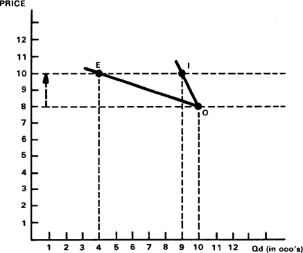
FIGURE 12:

ELASTICITY OF DEMAND IN THE CASE OF A PRICE-INCREASE.

Whether or not the $10,000 increase in TR is, in practice, enough to satisfy the firm, the fact remains that, technically speaking, the demand segment 01 is regarded as inelastic. Such “inelastic” responses are exactly what the firm would like to experience if and when it ever wants to raise its price, for only in such cases could TR be expected to increase in spite of the drop in Qd. In other words, the firm may be selling less but it is enjoying it more.

A Tableau of Our Results

Again omitted from our Figure 12 is the curious in-between category of elasticity technically referred to as unitary. As noted above, a “unitary” degree of elasticity is indicated only in those special instances where the price change somehow does not affect total TR even though the Qd changes; that is, TR remains virtually constant. In Figure 12 this unitary response would be indicated by a third dot placed right at the point joining the new $10 price and the reduced Qd of 8,000 units, which together make for a TR totalling $80,000—exactly the same as the original TR. Since the unitary response remains a relatively transitory case in practice, we will neglect it and devote our attention mainly to the more practically significant elastic and inelastic cases.

It is now possible to summarize the results of our analysis by the following tableau:

Type of Price Change	Change in Qd under Law of Demand	Change in TR as Indicator of Degree of Elasticity of Demand
Price Cut	+	+Elastic degree of elasticity -Inelastic degree of elasticity =Unitary degree of elasticity
Price Raise	-	-Elastic degree of elasticity +Inelastic degree of elasticity =Unitary degree of elasticity

Elastic vs. Inelastic: Which Is Better?

Before we proceed, we should explain some of the entries in the tableau: the “plus” sign indicates an increase in the Qd or TR, the “minus” sign stands for a decrease, while the “equals” sign stands for no-change. Now, the first thing to note is that elastic cases emerge only where the TR changes in the same direction as the Qd—that is, when TR increases while Qd increases, or when TR decreases while Qd decreases. On the other hand, the inelastic cases occur only when TR changes in a direction opposite to that of the Qd—that is, when TR decreases while Qd increases, or when TR increases while Qd decreases.

The next thing to note is that an “elastic” or “inelastic” demand does not always have the same practical significance for the firm. Thus, as illustrated by Figure 13, if the firm is considering a reduction of price, it would clearly prefer an elastic to an inelastic demand segment, since only an elastic demand will bring with it the desired increase in TR despite the price cut. Conversely, when the firm is considering a price increase, it would clearly prefer an inelastic demand segment, for only in this case will the TR increase despite the drop in Qd. Put another way, an elastic demand would be “good news” to the firm only when considering a price cut, while an inelastic demand is “good news” only when a price increase is being considered.

The Practical Importance of Demand-Elasticity

Once again, then, we see why knowledge of the law of demand is not enough as far as the firm is concerned. Of great practical importance is an awareness of the price-elasticity dimension of demand, especially as it operates through changes in TR. More precisely, only from its market experience can the firm learn, sooner or later, that elastic and inelastic demand segments will exert significantly different effects on TR when it undertakes a price change. Only through constant effort to adapt to changes in market demand, via adjustments in selling price and/or quantities supplied, can the firm learn anything about the elasticity of demand for its product.

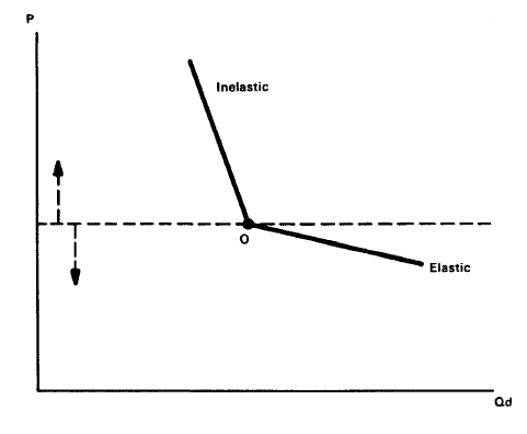
FIGURE 13:

DEGREES OF ELASTICITY PREFERRED BY THE FIRM.

By now, the preceding analysis must have raised at least two questions in the reader’s mind: (1) What are the various social, technical, and economic forces that help determine whether market demand will be elastic or inelastic? (2) In what ways can the firm acquire knowledge of the elasticity of demand, which can guide it in forecasting the possible effects of a price change? It is these two practical questions to which we devote the next part of this chapter.

II. The Determinants of Elasticity

In the following analysis of the determinants of elasticity, we enumerate and analyze several basic dimensions through which the forces influencing the degree of elasticity of demand exert their effects. These determinants of elasticity ultimately boil down to but a few basic dimensions having to do with the product itself, the nature of the competitive environment, and the subjective conditions of the consumer. Our analysis will help us learn the nature of those conditions which tend to make demand elastic or inelastic, and which are therefore of direct practical relevance to the pricing policies of firms. As we will see, there is nothing in this common-sense analysis that the firm cannot, and does not, learn from Its own trial-and-error experience in the market place.

(1) Availability of Close Substitutes

For virtually any given product X offered for exchange or sale in the market place, there can be found one or more close substitutes—other products that can serve the same purpose or provide the same utility (usefulness) as the given product X. One example already familiar to the reader involves butter and margarine (see Chapter VI). Substitutes need not be identical in physical properties. That is to say, the degree of substitutability or similarity of product is determined not only by the physical/technical properties of the interchangeable commodities, but also by the judgment of the consumer. Substitutability lies in the eyes of the beholder, so to speak.

If, for example, people use newspapers as well as wax paper for wrapping purposes, then this practice effectively makes them substitutes for each other with respect to the given purpose (wrapping), even though the two products are not physically identical. So long as the different products can be used to serve the same purpose, more or less, they are to that extent substitutable for each other—indeed, as far as the consumer is concerned, they may be viewed as rivals, in competition with each other.

Substitutes and Competition

Another equally important dimension of substitutability is the extent of competition provided by rival brands or firms producing the given product X. The larger the number of competing firms producing product X, the greater the degree of substitutability as far as the consumer is concerned. For example, if the consumer does not like Schlitz beer, for reasons of price or quality, he can find a half-dozen or more substitute beers produced by rival firms, all of whom offer a similar product that effectively serves as a close substitute for Schlitz.

We thus have not one but two dimensions of substitutability, both of consequence to the competition among products and firms. In effect, therefore, the availability of close substitutes is a reflection of the competitive environment facing the firm and its product. Hence, the greater the competition among both products and firms, the greater the availability of close substitutes—and vice versa. We now must ask: What is the effect of availability of substitutes on the degree of slope or elasticity of market demand? First, we will analyze the case of a price raise, and then the case of a price cut.

Substitutes and Elasticity

Assume, now, that a given firm has raised the price of its product, while other firms producing a similar product have not raised theirs, or have not raised theirs as much. It would be reasonable to assert: other things being equal, the greater the availability of substitutes, the more likely that the demand for the product will be elastic (see segment OE in Figure 14, part A); conversely, the smaller the availability of substitutes, the more likely that demand will prove to be inelastic (see segment 01 in Figure 14, part A). The reasoning here is straightforward: the greater the competition, the better able are buyers to locate relatively cheaper substitutes and to shift their purchases to those alternatives. They would rather switch than fight, to re-coin a phrase. Conversely, the smaller the extent of competition, the fewer the alternatives available to buyers.

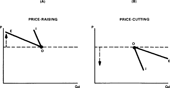
FIGURE 14:

PRICE-CHANGES AND PRICE-ELASTICITY OF DEMAND.

What about the case of a price reduction? Here it would be reasonable to assert the same propositions as in the case of a price increase: other things being equal, the greater the availability of substitutes, the more likely that demand will be elastic (see segment OE in Figure 14, part B), while conversely, the less the availability of substitutes, the more likely that demand will be inelastic (see segment 01 in Figure 14, part B). Here the reasoning would be as follows: if the ABC Company cuts its price while all other firms fail to follow suit, then the greater the extent of competition from rival brands and products, and the greater the number of customers that can be won over from competitors in favor of ABC’s lower price. Conversely, the smaller the extent of the competition, the fewer the customers to be won away from competitors.

Notice that in both cases of price raising and price cutting, the same conditions of substitutability result in the same degree of elasticity. Thus, the greater the availability of substitutes, the more likely that demand will be elastic in both the case of a price raise and a price cut. The same proposition applies to the situation where substitutes are not very available. As a consequence, the overall slope of market demand would be expected to be elastic (E) when numerous substitutes are available, and inelastic (I) when substitutes are not very available (see Figure 15).

Subway Fares and Oil Cartels

How does all this apply to the practical pricing policies of firms? A couple of important examples will suffice, although numerous others can be recounted. Officials of New York City’s subway system have been periodically faced with the need to increase their total subway receipts (TR), especially to finance increased wage demands by union workers. Which way should they go—reduce the subway fare or raise it?

History tells us that the subway authorities have repeatedly resorted to an increase in the fare instead of a decrease. Why? Presumably, officials ruled out fare cuts on the belief that demand would be inelastic for a lower fare: they were probably skeptical that they could attract enough additional subway riders by the lower fare. So they turned instead to the fare increase, implying a belief that they had an inelastic demand for transportation. Clearly, the millions of workers going to jobs every day in Manhattan and other boroughs have little alternative to the subway. The comparative absence of any serious competition from alternative systems of transportation—taxis and owner-driven autos—would make for low substitutability and inelastic demand. Since the subway TR was increased as a consequence, the hunch about inelastic demand proved correct.

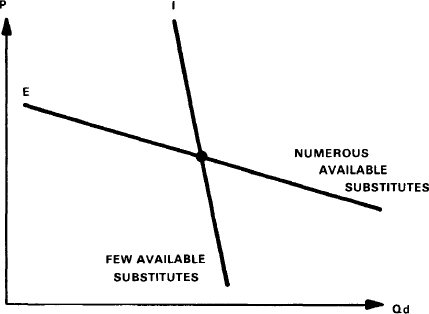
FIGURE 15:

AVAILABILITY OF SUBSTITUTES AND ELASTICITY OF DEMAND.

Another important example occurs in connection with the recent efforts of the oil cartel to increase total receipts (TR) by reducing supplies and charging higher prices. Intimately connected with this well-planned and orchestrated program were the gasoline “shortages” of the 1970’s and the accompanying significant increases in gasoline prices. The oil producers must have been very confident that their Western customers were not only heavily dependent on oil, but also had few available substitutes, at least in the short run. Economic studies confirm their judgment: they show, for instance, that the demand for gasoline in the U.S.A. is very inelastic.

Before we proceed to the next determinant of elasticity, it is important to remember the proviso in our propositions: “other things being equal,” i.e., ceteris paribus. This proviso reflects the fact that, in practice, there may be two or more determinants—not merely one—exerting their influence simultaneously on the demand for a given product. What makes this significant is the fact that the full array of determinants may not be exerting their influence all in the same direction, but rather in opposite directions. That is to say, one of the determinants may be imparting an inelastic thrust while another determinant may be imparting an elastic thrust. How does this affect our analysis of determinants? This will become clearer as we discuss other determinants.

(2) Relative Price of the Product

It is no secret that the various items we purchase in the market place have different price tags attached to them, and that some of these prices are relatively low or insignificant—such as the prices of newspapers, bottles of coke, or cigarettes—while other prices are relatively steep or expensive, such as the prices of automobiles or refrigerators. Even though automobiles and other durables may be bought on an installment basis, involving lower monthly payments, the fact remains that such payments constitute relatively large-size items in one’s budget. In any event, how would the relative dollar-size of the item affect the elasticity of demand?

The Case of a Price Increase

First, take the case of a price increase. For purposes of illustration, let us assume a price increase of 50 percent and compare the effects in the case of two differently priced products—say, a newspaper and an automobile. If the newspaper was selling for 20 cents, the new price would be 30 cents; if the car was selling for $6,000, the new price would be $9,000. Clearly, the impact on the elasticity of demand of the given 50 percent price increase would be vastly different in each case; the 10-cent price hike for the newspaper is virtually infinitesimal compared to the $3,000 boost on the car. As a consequence, a 10-cent boost would have virtually no deterrent effect on the rate of purchase compared to the deterrent effect of a $3,000 boost. Hence, it is reasonable to assert the following proposition: other things being equal, the smaller the relative price of the item, the more inelastic is the demand likely to be; conversely, the more expensive the item, the more elastic is demand likely to be—ceteris paribus.

This proposition can be confirmed by a variety of cases, but one important instance should suffice. A widespread practice among the governments of the world is the levying of excise taxes, particularly on low-priced items, such as cigarettes, cosmetics, movies, and liquor. This “nickel-and-dime” method of public finance has been a successful revenue raiser mainly because the low-priced items involved show inelastic demand against price increases. This means that the price hike caused by the tax has relatively slight deterrent impact on the rate of purchase.

The Case of a Price Cut

What about the case of a price reduction? Here, too, it would be plausible to assert the same proposition as above, and for similar reasons. A price cut on a low-priced item will spare the buyer only small amounts, and hence constitutes a relatively weak inducement to buy more. On the other hand, a similar percentage cut on a high-priced item will mean a relatively huge saving to the purchaser, and therefore constitute a very great inducement to buy. Hence, an inelastic response in Qd would be associated with the low-priced item while an elastic response would be expected in the case of a high-priced item, ceteris paribus.

Finally, we should note that, since our propositions are the same for both cases of price raising and price cutting, the overall conclusion is that elastic (E) demand will emerge in the case of high-priced items, and inelastic (I) demand will emerge in the case of low-priced items (see the slopes E and I in Figure 15).

The Meaning of “Ceteris Paribus”

Before we proceed to a third determinant of elasticity, it is pertinent to recall our earlier comment on the “other things being equal” proviso. There we noted that, in practice, we are likely to find not one but possibly two or more determinants of elasticity at work, and in opposite directions. Now, with the automobile, at least in areas where people have few alternative means of transportation (such as Los Angeles), we have an excellent example of this case.

In the Los Angeles area, for instance, automobiles are not only expensive in price (like everywhere else in the country) and in upkeep (because of the great mileage travelled by each driver), but they remain virtually the only means of transportation. (About the only substitutability is in switching from “gas-guzzler” models to “economy” models.) This heavy dependence on the automobile not only makes for inelastic demand, but also accounts for families tending to own two or more cars—depending on the size of family, etc.,—which further adds to the purchase expense. Thus, we have determinants of opposite influence on elasticity: on the one hand, the lack of available substitutes causes inelasticity of demand, while on the other hand, the great expense of acquiring cars makes for elasticity of demand. This makes it more difficult for producing firms to predict the overall effects of an increase in the price of new cars as well as an increase in the price of gasoline.

(3) Subjective Preference Ranking

At least twice before—in Chapters V and VI—we have met the subjective preference-scale on which, at any given moment, we rank our wants and the means to satisfy them. The specific forces that shape and influence these subjective preference rankings—the importance we attach to things—are as numerous and varied as the human mind can imagine. They include such widely ranging factors as individual nutritional requirements, aesthetic tastes, and lifestyle—on to advertising, fashion, and professional/technical requirements.

Price Increases vs. Price Cuts

Before we examine some noteworthy aspects, let us first state the following propositions. If the firm is contemplating a price increase, it would be reasonable to assert: other things being equal, the higher the subjective preference-ranking for the particular product or want, the more likely that the demand will be inelastic in the face of a price raise. (In this connection, see Figure 14, part A, segment 01.) Conversely, the lower the subjective ranking for the item, the more likely that demand will be elastic in the face of the price raise. (See Figure 14, part A, segment OE.)

The reasoning here is straightforward. The more important the item is for the consumer, the less resistant will the consumer be to a price increase—ceteris paribus. The example of gasoline readily comes to mind. The inelastic demand attributed to gasoline in the face of price increases is as much due to the importance attached to the automobile as to the lack of available substitutes for automobile power. Conversely, the less important the item is for the consumer, the more likely that he will be deterred from buying at the higher price—other things remaining the same.

What about subjective preferences and price reduction? Here the propositions would run as follows: other things being equal, the stronger the subjective preference, the more will demand tend to be elastic, while the weaker the subjective preference, the more likely that demand will be inelastic. (See Figure 14, part B, segments OE and 01, respectively.) And the reasoning here is also straightforward: the more important the item is to consumers, the more likely are they to take advantage of the price cut; the less important the item, the less likely are consumers to be induced to buy by the price cut.

Practical Implications

A further significant proposition follows from these considerations. On the assumption that firms prefer larger total receipts (TR) to smaller TR’s, they will tend to produce goods of higher-valued preference, or cater to wants of higher rank, rather than produce goods or cater to wants of lower-valued rank.

In this connection, an examination of Figure 16 readily tells us why: higher-ranked goods or wants (see part A of Figure 16) are associated with demand segments whose degree of elasticity implies increased TR’s if and when the firm wants to either increase its price (see segment 01) or cut its price (see segment OE); conversely, lower-ranked goods or wants (see part B of Figure 16) are associated with demand segments whose degree of elasticity implies decreased TR’s when the firm raises its price (see segment OE) or cuts its price (see segment 01). To put it another way: if ever the firm is faced with the decision to change its price in order to increase its TR, it would clearly be better off producing goods of higher value than goods of lower value.

The Case of Agricultural Products

All of this has great relevance to government policy on agricultural products—their supply and pricing. Here it suffices to note that the demand for agricultural products and foodstuffs as a whole is overall inelastic. This means that farmers face two alternatives. They could, on the one hand, increase their TR’s by producing less and charging higher prices. On the other hand, they could increase production and reduce prices in order to increase the Qd; but in so doing their TR’s would decrease due to the inelastic demand!

At least two interesting implications emerge from the agricultural case. One is the implication, just noted, that farmers can be induced to increase their TR’s by producing less and increasing prices. The other is an implication that applies to other goods that share a similar characteristic: while these goods possess great importance for people, they are nevertheless needed in only minimum quantities, such that the demand for them is inelastic both for a price raise and for a price cut.

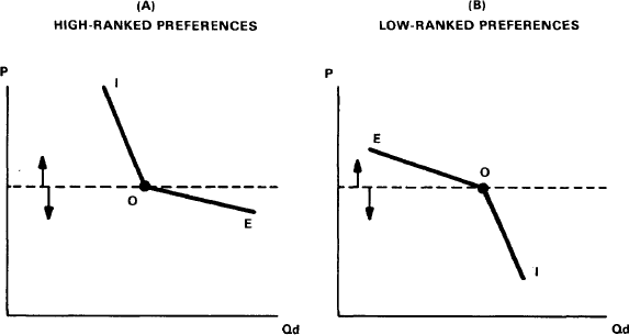
FIGURE 16:

PREFERENCE-RANKING AND ELASTICITY OF DEMAND.

Minimum Requirements

For example, in the case of foodstuffs, people generally desire certain minimum quantities for nutritional purposes (causing demand to be inelastic against a price hike). For this reason, they are not sufficiently attracted to opportunities to acquire more foodstuffs at lower prices, in preference to other goods (hence the inelastic demand to a price cut). Similar is the case of special technical instruments or equipment, such a slide-rules, pocket computers, or stethoscopes. For these items, people have only a limited professional or technical requirement—that is, they need but one unit, not more. Therefore, the firm would have to cut its price steeply in order to induce buyers to acquire a second unit or more. It may be noted, however, that at the greatly reduced price, additional customers can be picked up from two other groups of purchasers: people who have a relatively low-ranked preference for such items, and can be induced to buy only by a much-reduced price; and people in lower-income classes who can now afford to buy at the much lower price. This latter dimension of elasticity-determination will be examined in more detail in the next section.

(4) The Structure of Social Income

This dimension of demand-elasticity is relevant primarily to two cases. One involves a given product that has significant markets in each of the layers of the social income structure—from the higher-income strata, down through the middle-income, and into the lower-income strata—such that the problem facing the firm involves a judgment as to which price or price range will maximize its total receipts (TR).

Other things being equal, a relatively high price caters primarily to upper-income people, but because their number is comparatively small, the quantity demanded by them will be relatively small (see the relevant inelastic segment of the demand schedule in Figure 17). On the other hand, a relatively low price caters primarily to lower-income groups, but since they exist in greater numbers, their Qd may be considerably large (see the elastic segment of demand in Figure 17). As a consequence, the firm must decide which of the two attractive segments of the market offers the comparatively greater TR, assuming the costs of producing the two different quantities does not significantly affect the pricing decision.

Closely related to this type of decision—which involves the question: Which level of price will maximize the firm’s TR?—is another practical question: Which level of quality or grade of product will tap the most lucrative markets? Generally speaking, people associate higher prices with higher-quality products, and lower prices with lower-quality goods. Thus, assume an automobile producer who is able to turn out either a very expensive, high-quality, deluxe car (with a relatively inelastic demand) or a relatively inexpensive, lower-quality, mass-produced car (with a very elastic demand). The one car would cater to a select group of rich people or car enthusiasts; the other car would tap the untold riches of the mass market. If an entrepreneur were motivated primarily by the vision of a potential mass market, he would clearly undertake production of the inexpensive, mass-market car. Could this have been the paradigm for Henry Ford and his Model T car?

(5) Supplies On Hand in the Pantry

In pursuing this catalogue of elasticity determinants, we should also note a factor that must be presumed to be an important influence on elasticity, but its significance cannot be easily ascertained by the firm. It involves a wide variety of storeable commodities (from canned goods and linens to gasoline for the car), which are kept in consumers’ refrigerators, freezers, pantries, closets, tanks, attics, or wherever. Typically, the quantity or stock in possession of the consumer can vary from zero or low to full or ample, so that the firm cannot gauge the state of consumer inventories of consumables with sufficient precision. Nevertheless, the law of marginal utility (Chapter V) enables us to assert the following propositions.

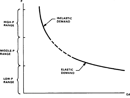
FIGURE 17:

SOCIAL INCOME STRUCTURE AND ELASTICITY OF DEMAND.

First, the case of a price increase. Other things being equal, the greater the quantity of goods already in consumers’ stocks, the more likely that consumers’ demand will be elastic in response to the price-hike; conversely, the smaller the stocks on hand, the more likely that consumers’ demand will be inelastic rather than elastic. The reasoning, based on the law of marginal utility, would run as follows: with ample or bulging stocks on hand (and the law of diminishing MU therefore becoming relevant), consumers would be less inclined than otherwise to pay a higher price; with small or meager supplies on hand (and the law of increasing MU therefore becoming relevant), consumers would be less deterred than otherwise from buying at the higher price.

A parallel line of reasoning applies to a price reduction. Other things being equal, the greater the quantity in consumers’ stocks, the more likely that consumers’ demand will be inelastic in response to the price cut; conversely, the smaller the stocks on hand, the more likely that demand will be elastic. Why? In the case of ample stocks on hand, the law of diminishing MU becomes relevant: the lower price is less of an inducement to buy than otherwise. However, when stocks are very low, and the law of increasing MU becomes relevant, the consumer finds the lower price a greater inducement to buy than otherwise.

Complexity of Determinants

As a concluding note to this analysis of elasticity determinants, it is necessary to stress again that, in the real world, these determinants may exert their influence in combinations of two or more simultaneously, but with mutually opposite impacts on Qd. What we have done in this part of the chapter is a “partial analysis”—a study of the effects of isolated or particular forces at work, on the ceteris paribus” assumption that other influences are not simultaneously at work. This enables us to explore theoretically the full workings of any single factor. Then, equipped with this knowledge of the workings of individual determinants, we should be better able to forecast the effects on elasticity that may be exerted by the complex, real-world conditions facing the firm in a given market.

In this connection it is important to recall (from Chapter VI) that the firm knows little, if anything, about the demand schedule for its product—other than its current “dot,” that is, its current selling price (P) and the quantity demanded (Qd) at that price. The only other thing the firm knows is that there is a demand schedule out there in the market—albeit unknown—and that if the firm raised (or lowered) its price, the Qd would decrease (or increase).

Demand—The Unknown

But surely this is not enough. The firm could still not know in advance by how much the Qd would decrease (or increase) when it raises (or lowers) its price. Indeed, such information about the effect of a price change cannot be known until the firm actually institutes the price change. Even then, the firm would discover the degree of elasticity pertaining to only one segment of a potentially more complete demand schedule. Logically, the only way the firm could discover the full array of “dots” constituting the demand schedule would be to conduct a kind of experiment: It could post a series of price changes over a wide range in order to uncover the full array of the respective P and Qd dots that comprise the demand schedule—assuming, of course, that the demand schedule does not shift throughout the entire experiment!

In practice, however, firms cannot and do not play such games. They do not change prices unless provoked by special circumstances. For instance, they have in the past raised prices mainly in response to rising costs rather than to take advantage of increased demand; from the public relations viewpoint, they prefer not to be accused of “charging what the traffic will bear.” Conversely, they reduce prices mainly under the pressure of increased competition or the need to dispose of overpriced goods.

III. Some Important Questions

Can firms charge just any high price they want, and still prosper? Do firms always charge the highest price consistent with maximum profits? Do firms actually have complete knowledge of market demand so that they know exactly which price will maximize their profits? These and related questions can be answered, at least partly, with the help of the demand-elasticity concept. Let us see how.

The Firm as “Profiteer”

There is a widespread notion that, if left alone, the firm would automatically charge the “highest possible price” simply out of rapacious greed, and that only fear of government reprisal (e.g., anti-trust action by the Justice Department) keeps it from resorting to price “extortion” or “profiteering.” Whether or not it is true that fear of public reprisal keeps the firm in check is strictly an empirical question, which may or may not be open to investigation. As far as economics is concerned, the market alone suffices to keep prices of firms in check (as we will see especially in the next chapter); it would be a waste of valuable resources to set up a public agency merely to police prices in the market place when, all along, the market itself can serve this function.

It should be noted here, however, that no firm in its right mind would blindly and steadily raise prices regardless of the elasticity of demand for its product. As we have amply seen, the only time it pays the firm to raise its price is when market demand is inelastic (not elastic!), for only inelastic demand will yield an increase in total receipts (TR) and an increase in total profits. (This assumes that cost-changes are not a factor—that the smaller production rate due to the drop in quantity demanded (Qd) does not affect total costs in a way that affects the profit rate.) However, if, following the price raise, demand proves to be elastic, the result would be a drop in TR and (assuming no cost-effects) a drop in profit rate, too, which should suffice to check the price-raising! In other words, the firm would go for a price raise only as long as demand is inelastic; if demand turns out to be elastic, the price-raising will stop.

Ex-Ante Ignorance

This brings us to a related question. Assume a firm that, in quest of increased TR and believing market demand to be inelastic, decides to raise its price. And lo and behold, it discovers it guessed correctly—its TR actually increases. This prompts the question: How come the firm had up to now been asleep at the wheel—selling at a lower price and TR—when all along it could have been selling at a higher price and a larger TR? Assuming costs of production were not a factor, it looks like the firm had up to this point foregone higher profits. Why would it do so?

One possible answer is that the firm was more or less ignorant of the degree of elasticity of market demand when it had made its original ex-ante decision—when it set the price at, say, $10 in the belief that this represented its most profitable price for the quantity produced. Had it known originally that a higher price of $12, say—and a smaller quantity of production—would have brought a higher TR, it would undoubtedly have opted for that combination of P and Q. But in view of its ignorance—its incomplete knowledge of the actual demand situation—it could not know in the ex-ante what it could know only in the ex-post, after trial-and-error. (See Chapter V on maximizing and the ex-ante/ex-post aspects of decision-making.) In other words, had the firm at the start possessed perfect knowledge of the market demand, it would have opened up with a $12 price—it would never have had to raise its price from $10 to $12, and consumers would not have any grounds to complain of “profiteering”!

“Social Pressures,” Competition, and Income Changes

Another possible reason why a firm might only belatedly discover that its initial price had been set too low—in the sense that it was less profitable than the higher price it set later—is the widespread reluctance of firms to raise prices in the face of various “social pressures.” One such pressure stems from the taboo, already mentioned, against “charging what the traffic will bear.” In terms of elasticity this means: do not raise prices even though demand is inelastic and TR would increase! Another form of pressure stems from the fear of prosecution by the Justice Department under the anti-trust laws, on the grounds of “monopoly” or “market power.”

A third possible reason is the firm’s fear of competition from rival firms and rival products, such that a price raise might leave it out on the limb—losing customers to rivals that had not raised their prices. In such cases it might occur to the firm that the best way to achieve higher profits is through collusion with its rivals. Such concerted action would involve a basic agreement among firms to restrict supply, rig prices, and bolster profits by means of pools, mergers, or cartels. In other words, the firm may overcome its fear of competition by, in effect, outlawing it in concert with its rivals. But history tells us that such cartel-like arrangements have never worked without the backing and legal sanction of government.

A Note on Cartels

In this connection, history also reveals that cartels organized by commodity-producing nations—in order to restrict supply and maintain the price of copper, coffee, oil, etc.—have tended to underestimate the degree of elastic response in consumers’ demand as a consequence of consumers’ ability to find substitutes in the long run. Indeed, all demand schedules possess some degree of elasticity due to the availability, more or less, of substitutes.

History reveals that in the long run there is no such thing as a totally vertical (totally inelastic) demand schedule. Man has not let himself be crucified by a price hike. He has had the ingenuity to use science and technology to find those substitutes that enable him to reduce reliance on higher-priced resources. And this is probably the most productive as well as the most effective way of bringing any cartel to heel.

Rising Incomes and Price-Increases

Also worth mentioning is the following peculiar situation. Imagine a case in which TR increases at the same time that the firm raises its price—but not as a result of inelastic demand. This is the case where market demand had increased at the same time that the firm had raised its price. In this case, the firm may not have realized that demand had increased because personal incomes of households had increased, thereby causing a “shift to the right” in the demand schedule (see Chapter VI). In this case the TR is increased not because of inelastic demand but because, despite the higher price, the increase in the demand schedule was sufficiently large so that the Qd remains undiminished or even increases!

Why Not Blame the Consumer?

The fact that the firm can raise its price and increase its TR raises another issue. There have always been people who regard price-raising by the firm as “reprehensible” or “gouging.” Since it is usually inelastic demand that enables the firm to earn a larger TR when it raises its price, two further questions become very relevant: (1) Why blame the firm for inelastic demand, when only the consumers are ultimately responsible for that? (2) Does not the firm have the right to take advantage of a market situation which reveals an inelastic demand for a given product?

As to the first question, it should be noted that whereas consumers—not firms—should be blamed for creating the inelastic demand, these same consumers have it in their power to reverse the situation and create an elastic demand—simply by sitting on their hands and curtailing their spending! Therefore, if consumers think a firm’s price and TR are “too high,” and really want to bring them down, nothing stands in their way but their resolve to buy less.

A Question of Human Rights

As to the second question—concerning the firm’s right to maximize its profit by increasing its TR—it suffices to note that it involves a moral issue. Virtually all attacks on the firm that concern their pricing and production policies—e.g., the firm’s price is alternatively “too high” (“extortion”!), “too low” (“price warfare”!), or the firm is alternatively producing “too much” (beware of “growth” and “affluence!”), or “too little” (“monopolistic restriction”!)—these attacks are not only self-contradictory but also boil down to questions of fundamental human rights. Does a person have the right to ask any price he wishes for his goods and services? Does he have the right to produce as much or as little as he desires? These fundamental questions will turn up again in Chapter X, wherein we analyze the nature of a free-market economy.

 

Appendix

THE COEFFICIENT OF ELASTICITY

It is not usual to give the concept of demand-elasticity a whole chapter all to itself as we have just done. Nor is it usual to treat elasticity in “TR” terms, although textbooks are tending more and more to do so. More usual, because it is traditional, is to describe elasticity in “percentage” terms—that is, to compare the percentage change in quantity-demanded with the given percentage change in price. The purpose of this appendix is merely to alert the reader to the existence of this alternative concept, which he can pursue in greater detail in any introductory or intermediate textbook.

Theoretically, there is no basic conflict between the TR approach and the percentage approach; they are two different ways of looking at the same thing. In the percentage approach, the criterion of elasticity is referred to as the “coefficient of elasticity,” which is derived as follows:

Thus, the COE turns out to be a number that reflects the numerical relation or ratio between the rate of change in P and the rate of change in Qd. The plus or minus signs that are involved mathematically can be conveniently disregarded for the purpose of calculating the COE.

Let us take a simple example. Suppose a price cut of 15 percent results in a 20 percent increase in Qd. The resulting ratio is 20/15, equivalent to 1-1/3, or 1.333. Since any COE that is numerically greater than 1.0 is classified as elastic, the above case reveals elastic demand. Another simple example: suppose a price raise of 20 percent results in Qd dropping only 10 percent. Calculation yields a ratio of 10/20, equivalent to 1/2 or .5. Since any COE that is numerically less than 1.0 is classified as inelastic, we have here a case of inelastic demand. Finally, the unitary case arises where the percent changes in Qd and P are exactly equal, yielding a COE of 1.0, the standard for unitary elasticity.

Notice that both the TR and percentage criteria involve the same basic elements: P and Qd. But the TR figure, compared to the COE, has the advantage of not requiring any further calculation once the raw TR data have been statistically adjusted to eliminate the effect of non-price influences on TR—a statistical procedure that is also required in calculating the COE. In contrast, the COE requires the further calculation of the respective percentage changes in P and Qd, and then the ratio of these percentage changes.