
Common Sense Economics
Part I. The Stationary Economy
The Isolated Producer
Everybody tries to live. In order to live one has to consume goods. Goods for consumption are not generally obtainable without work. They are the products of labor. This holds true for individuals, for communities and for the whole of humanity.
When somebody produces consumption goods by his own work he exchanges, so to speak, work-hours, of which he has plenty but which he cannot consume directly, for goods which he can consume but which he lacks until they are produced. This is exchange in its simplest form. We have to understand it thoroughly in order to understand other forms of exchange which, though somewhat more complicated, are all based upon the same principle.
Our ability to exchange work for goods, to produce, rests upon the fundamental fact that nature offers the technical possibility of transforming work into goods—say of transforming one hour of work into ten apples. Given this technical possibility there arises the question of how many hours men will actually use to produce the apples they wish to consume. The answer is that each individual decides how many hours of leisure he is willing to sacrifice in order to satisfy his appetite for apples. It is up to each individual to decide when the point has come at which the disutility of work is no longer compensated by the utility gained by more apples.
If a man considered the utility of every additional apple, as compared with the disutility of every additional hour’s work, to be the same as that of all previously acquired apples and previously worked hours, he would obviously work himself to death—provided he started out by wanting any apples at all. He would be killed by an insatiable appetite for apples and a flagrant disregard for his physical limitations. He would never stop working, and we could never know his relative valuation of apples and work-hours.
Fortunately this never happens. The famous law of diminishing marginal utility, or better, the law of diminishing valuation of additional quantities of goods, comes into play. The utility of each new apple which even the most passionate lover of apples acquires appears to him less than the utility of apples previously produced. On the one hand the need for apples becomes less pressing and is finally limited by the individual’s consumption capacity. Even utmost greed is satisfied. On the other hand the remaining rest and play hours become fewer and therefore more urgently needed. The individual’s valuation of leisure increases. This means that our man will demand an increasing amount of apples for each additional work-hour; or, looking at it from another angle, his supply price of work in terms of apples will be higher for every additional hour. If the working day is to lengthen, nature must pay him a higher price for each working hour. Inevitably the price at some point will be more than nature can pay.
Our man may be prepared to work one hour each day in return for only two apples. This one hour is needed neither for rest nor for play, whereas he values the apples highly because they are his first. He may be willing to work the following hour for a return of four apples, the next for six apples, and so on. The eighth hour, maybe, he will sell only for a return of say sixteen apples. He may not be prepared to work at all the ninth hour, even for much greater compensation, because his appetite for apples may be satiated by those already obtained and his desire for rest may have become very urgent.
It is usual to represent willingness to supply work by a graph in which the quantities offered are measured on the horizontal axis, and the price at which they are offered on the vertical line. The resulting supply curve then slopes upward from the left to the right.
The assumptions referred to above can thus be represented by the supply curve shown in Figure 1.
The supply curve slopes upward to the right up to the eighth hour. It shows how the hours of work offered increase with the price paid. From the eighth hour onward the curve rises vertically: the supply of work-hours no longer increases with rising prices. No matter how much the price is raised it no longer has the power to lengthen the working day.
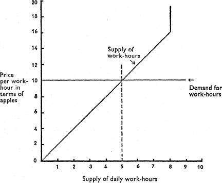
FIG. I
Our assumption that until the eighth hour the supply of labor increases with the wage demanded is broadly in conformity with reality. According to the general law, the higher the price the greater the supply.
In the particular case of labor supply, however, we must note a peculiarity. A higher wage level, and the resulting higher living standard of the workers, may cause a change in their value judgments. The workers may prefer additional rest to additional consumption goods. We then speak of the supply curve of labor moving upward or to the left. This indicates that less work is now forthcoming at each of the various compensation levels. On the other hand when the wage level, and with it the living standard, falls the workers may prefer to have more consumption goods rather than more rest. The supply curve of labor then moves downward or to the right, indicating that more work is forthcoming at each of the various compensation levels. This renders the effect of wage changes somewhat unpredictable, especially in the long run. History shows that the higher wages resulting from the increased productivity of the economy have been used by labor partly to increase leisure and partly to buy more goods. In insisting on shorter working time labor went without a certain amount of consumption goods which it could otherwise have obtained. We shall, nevertheless, assume that in the general case higher wages lead to an increase in the supply of work-hours.
Let us return to our diagram. How many hours will our man actually work on the assumption underlying our curve? The answer obviously depends upon the price, in terms of apples, which the demand for labor is prepared to pay. In our simplified model it is nature herself who demands labor in exchange for apples. But nature, working neither at a profit nor at a loss, offers for a work-hour exactly what an hour’s work produces. Suppose this is ten apples. Then nature offers ten apples as a reward for every hour of work. We represent this demand situation in our graph in the usual way by a horizontal line at the wage level of ten apples an hour. We immediately see that on the given assumptions our man will work five hours and produce fifty apples—not more and not less—because nature’s offer of ten apples for an hour’s work is exactly the compensation which our man demands for his fifth hour. In other words his work stops at the so-called marginal work-hour where the price, at which its supply is offered, is still just covered by the price which the demand is prepared to pay.
Some Preliminary Consequences
This is, of course, a very simplified model of what would happen in the real world even within an isolated economic unit. Yet for all its simplicity it shows quite clearly certain fundamental facts about the economic world which we will encounter again and again as we proceed to the examination of the more complicated real conditions:
(1) Production never expands beyond the point where the worker demands more for his work-hour than he produces during this work-hour. Any expansion of production depends upon the worker not demanding more in payment than he produces.
(2) At a given schedule of prices at which the worker offers various quantities of work-hours, that is at a given particular supply curve for labor, production can expand only if the productivity of labor increases. Higher productivity of labor enables nature to pay greater compensation, in terms of product units. The extra-marginal work-hours, which had so far been too expensive, can now be used.
In our model the work-hours were supplied by one single worker. If there are several workers it is now possible also to use work-hours of other workers, who had so far not been employed at all because even their first hour was too dear. Higher productivity, therefore, leads not only to longer working time for individual workers, but also to the employment of more workers.
(3) At given productivity of labor, and hence given demand for labor, production can expand only if the supply price of labor decreases. This will happen if the workers either value the utility of consumer goods more or the disutility of work less than they did in the past. Workers will then offer the same amount of work at lower prices, or more work at the same prices. Individual workers’ hitherto idle hours or hitherto idle workers will be drawn into the productive process.
This means that a population can consume more if it is willing to work more and to rest less. This truth is often forgotten nowadays, although it is self-evident to common sense. The comparatively low living standards of tropical countries are admittedly at least partly due to their peoples’ greater appreciation of rest and lesser appreciation of the comforts of life to be produced by work.
(4) The over-production problem, one of the major problems that has intrigued economists, does not exist in our simplified Robinson Crusoe world. So far as it occurs in reality, overproduction has its roots in conditions not present in the case of the isolated producer. Here there can never be separate decisions on consumption and production. Production and consumption are so closely linked that neither can ever exceed the other. Never can anything be produced that is not consumed. Jean-Baptiste Say’s law, according to which any production creates a corresponding consumption, is unconditionally valid. As soon as the utility of consumption goods no longer compensates for the disutility of the work of producing, production stops.
(5) Our model also allows us to make certain preliminary remarks on the important subject of profits. Our man receives a uniform compensation of ten apples for his work-hours, although it is only for the fifth hour that he demanded this compensation. He demanded substantially less for the first, second, third and fourth hours. He receives in fact more than what he considered sufficient to compensate him for his work. This is his good fortune and results from the fact that nature, exercising demand for his labor, values one work-hour at ten apples. For this reason nature pays, for all hours, more than the minimum compensation which he required for his first intra-marginal work-hours. But this surplus is not a profit in the usual sense of the word.
A profit is a phenomenon of distribution. It is a surplus arising when part of the output is withheld from other production factors for special reasons. No such surplus exists in the case of an isolated producer. His own input (of work-hours) is always both necessary and sufficient to produce the whole output (of apples). The two are always equal, and neither can exceed the other. Even if more is produced through improved techniques, there will still be no surplus, A given input can always result only in the output corresponding to the technique employed. If our man were to save or hoard his output, the apples, he would indeed end up with a stock of apples. But this would be not because he had made a profit from his production but because he had saved or hoarded part of the output.
An isolated producer can never make a profit, nor as we shall see later (p. 16) can an economy as a whole. We shall have to keep this in mind in our later examination of the true nature and origin of profits.
A Multitude of Products
We have so far assumed that our man has the choice only between rest and producing a single product, apples. In our example he was prepared to work five hours to produce fifty apples.
We now take a small step away from the simplest model of economic life toward the enormous complexity of the actual economy by assuming that he can produce and consume more than one product. In order to simplify the presentation, however, we shall assume that our individual has only the alternative of producing and consuming one more product, pears. So far it was a choice between rest and work; now there is the additional choice between the production and consumption of several goods. In analyzing the basic principles of this choice we are faced with one of the most important problems in economics—namely the problem of how mankind allocates available resources to various possible productions.
In our example our producer worked five hours to achieve a total production of fifty apples. Let us suppose that he wants to work neither more nor less than before. To what extent will he replace the production and consumption of apples with those of pears, now that he has the choice between the two? The answer depends on the one hand upon his valuation of the relative utilities of pears and apples, and on the other hand upon the relative production costs of apples and pears. The question arises whether more or less time is needed to produce pears rather than apples.
When the choice is between work and rest, the utility of the products of work is, as we have seen, valued exactly according to the law of diminishing marginal utility: the utility of additional apples appears less as their number increases. The same law governs the decisions relating to the consumption of two products, apples and pears. Our man will, therefore, value pears lower in relation to apples, as soon as the quantity of the former increases. This also because the utility of apples now appears greater to him. For if we assume that our producer wishes to produce pears only by sacrificing some of the time hitherto employed in the production of apples, the latter become scarcer.
Our man might, for instance, consider the utility of the first 5 pears as equivalent to that of 15 apples (1 pear = 3 apples); the utility of the next 5 pears as equivalent to that of 10 apples (1 pear = 2 apples); and the utility of the next 5 pears as equivalent to that of 5 apples (1 pear = l apple). The next 5 pears might drop in his valuation to less than 5 apples.
These valuations are, of course, the result of the psychological fact that the appetite for pears decreases with increasing satisfaction, whereas the appetite for apples increases with decreasing satisfaction. We are assuming that the individuals are aware of this fact when making their production plans for a certain time period.
Anyone who is prepared to forgo apples if he can produce pears instead, demands from himself, as it were, pears in exchange for apples. The valuation of pears in relation to apples can, therefore, be represented by a demand curve in the usual way. On the assumption just mentioned, this curve will have the shape pictured in Figure 2.
It has become usual in recent years to present the distribution of a given income (or effort) between two consumption (or production) possibilities with the help of so-called indifference curves. Since this technique is generally less accessible to laymen than simple demand and supply curves, we have tried to do without it, especially as we believe that the introduction of the indifference curve technique does not involve any substantial change or progress. The method of presentation adopted here reaches essentially the same results.
Now how many pears will actually be produced, and how many apples sacrificed? This obviously depends upon the supply of pears. Pears are, so to speak, supplied by nature when work previously devoted to the production of apples is transferred to the production of pears. The supply of pears in terms of apples is, therefore, dependent upon the relative production costs of apples and pears—in other words upon how much more or less time it takes to produce pears rather than apples.
Our graph with its several supply curves shows how many apples and pears our man will produce, provided the assumptions underlying the demand curve remain unchanged.
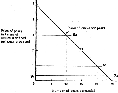
FIG. 2
If we assume that it takes the same time to produce pears and apples, the horizontal supply curve is situated at the price of one apple, or curve S1. If it takes three times as much time to produce a pear as it does to produce an apple, the horizontal supply curve will run at the price of three apples, or curve S2. If to produce pears takes one-third of the time that it takes to produce apples, the supply curve will run at the price of one-third of an apple per pear, or curve S3. The position of the intersection points between the demand curve and the three supply curves immediately provides the answer to the question of how many pears and apples will be produced on our various assumptions. In the first case (represented by S1), our man produces 20 pears and sacrifices 20 apples in order to do so. Instead of having 50 apples he will now have 30 apples. In the second case (represented by curve S2), 10 pears are produced at a sacrifice of 30 apples. Instead of 50 apples there will now be 20 apples. In the third case (represented by curve S3), where only one-third of an apple need be sacrificed for the production of each pear, 23 pears will be produced at a sacrifice of nearly 8 apples. Instead of the original 50 apples there will now be 42.
Differences in Utility Judgments
We have so far been analyzing the behavior of a single producer or Robinson Crusoe. However, an economy does not consist of a single producer but of innumerable producers. If all made the same value judgments and produced goods at the same costs—meaning, in our simplified model, that each producer would be devoting the same number of hours of work to the production of the same goods as every other producer—then the output of all producers would have the same composition. The whole economy would be no more than the sum of all the similar, even if separate, activities of its members. No new problem would arise. But men do not all have the same tastes, nor do they all produce the same goods with the same expenditure of work-hours.
Let us, therefore, turn to an examination of an economy with more than one single producer-consumer. For simplicity’s sake we assume that there are two, A and B. Our single producer valued pears in terms of apples in the manner shown in Figure 2. Suppose that the value, in terms of apples, which A attaches to pears is less than our single producer’s. Producer B, on the other hand, attaches greater value to pears in terms of apples than did our single producer. This situation is pictured in Figure 3. The curve Da (A’s demand for pears in terms of apples) now runs to the left of curve D, the demand curve of our single producer. The demand curve Db of producer B runs to the right of the former demand curve D.
We can now immediately see how many apples and pears A and B produce, if we assume that the production costs of apples and pears are the same (supply curve S1), and if we also assume that the original work-rest choice remains valid, i.e. that each works the number of work-hours that is required for the production of 50 apples. A then produces and consumes 15 pears and 35 apples, while B produces and consumes 25 pears and 25 apples. Our single producer produced and consumed 20 pears and 30 apples. A now concentrates more on the production of apples, B more on the production of pears. Even though the production costs of pears, in terms of apples, are the same for both, differences in taste have resulted in a different proportion of pears to apples in each of the two producers’ total output.
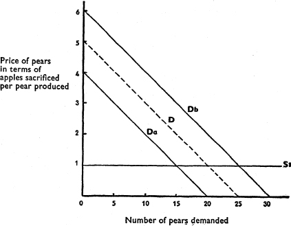
FIG. 3
Differences in Production Costs
We can now take another small step towards reality. It is most unlikely that production costs will be the same for two or more producers. Differences in the ability to produce various goods may be the result of tradition (a man learns the art of producing apples from his father), or of natural conditions (apples grow better on his land than pears). But whatever the reasons, the fact remains that the cost of production of goods in terms of work-hours normally is different for different people.
Figure 2 has shown us what a single producer would produce and consume at various production cost levels, given a certain demand curve, i.e. a certain judgment of the comparative utilities of apples and pears. Suppose now that A can produce pears only at higher cost, i.e. by more work, than B. A may, for instance, be working under conditions represented by the supply curve S2 in Figure 2 (1 pear can be produced by sacrificing 3 apples), while B may be working under the conditions of supply curve S3 (1 pear can be produced by sacrificing 1/3 apple). If the demand curve for A and B were that of our original single producer (D), producer A would now do as the single producer did when faced with supply conditions S2, i.e. produce 10 pears and 20 apples; at the same time producer B would do as the single producer did when faced with supply conditions S3, i.e. produce 23 pears and 42 apples.
But the demand curves of A and B differ from those of our single producer; the demand curves now are as Da and Db in Figure 3. To demonstrate what will happen, we have only to amalgamate Figures 2 and 3 in Figure 4, which shows: Producer A, with demand conditions Da and supply conditions S2, produces 5 pears. To do so he must sacrifice 15 of the original total of 50 apples, leaving him with 35 apples. Producer B, with demand conditions Db and supply conditions S3, produces 28 pears at a sacrifice of just over 9 apples, leaving him with nearly 41 apples. A thus produces only 1 pear for every 7 apples—a result of his being both a man with a weaker taste for pears and a poorer producer of them. B produces just over 7 pears for every 10 apples, the result of both greater liking for pears and greater proficiency in their production.
Exchange of Goods
So long as both A and B produce at the same cost, each sacrificing the same number of working hours for the same quantity of the same product, no exchange takes place between A and B no matter how different their individual relative valuations of apples and pears may be. Production simply follows the demand and consumption of the individual producers. But if the production costs of A and B differ, exchange will take place as soon as they are no longer isolated from each other but able to exchange goods.
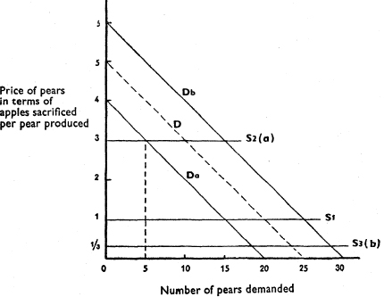
FIG. 4
As an isolated producer, A could produce 5 pears only by exchanging 15 apples with nature, since his production costs for pears are those shown by curve S2 in Figure 4 (1 pear for 3 apples). It would obviously be advantageous for him to produce no pears at all but only apples, and to exchange some of the latter for pears with B, whose production costs for pears are those shown by curve S3 (1 pear for 1/3 apple). So-called division of labor would be the result. No one any longer produces everything. Labor is divided according to what is to be produced. It should be noted that in our example both A and B produce apples at the same cost. What differs is the production cost of pears in terms of apples. It is the difference in the relative production cost of apples and pears which makes exchange advantageous.
How could an exchange of products between A and B be made under the cost condition described? We see that A produces 1 pear in the time it takes him to produce 3 apples, and that B produces 3 pears in the time it takes him to produce 1 apple. The most advantageous exchange for A would be to receive 3 of B’s pears in exchange for each of his own apples; and the most advantageous exchange for B would be to receive 3 of A’s apples in exchange for each of his own pears. Both exchanges are possible, but in either case only one of the producers would gain; by an exchange at any level in between both producers could gain.
If A gives less than 3 apples for each pear he receives, he gains by the exchange, for his production costs are such that he must sacrifice 3 apples for every pear he produces. On the other hand, if B receives more than 1 apple for every 3 pears, he also gains by the exchange, for in his own orchard he must sacrifice 1 apple for every 3 pears he produces. The range within which exchange is advantageous for both producer A and producer B is therefore between 1/3 and 3 apples per pear, or between 3 and 1/3 pears per apple.
The actual exchange rate of apples for pears at which the deal will go through depends, in our two-producer economy in which there are no competing parties in the market, upon the respective bargaining ability of A and B. All that can be stated with certainty is that the rate is bound to be within definite limits, and even that is contingent upon a rational behavior of both producers—meaning that both try to maximize the advantages to be obtained.
Let us assume that the price of pears expressed in apples will be somewhere between the two extremes, say 1 apple for 1 pear. How many apples and pears will A and B produce and eventually consume? According to Figure 4 producer A obtained his 5 pears by sacrificing 15 apples. The possibility of exchange with B, whose production cost of pears in terms of apple production time is lower, makes it advantageous for A to obtain his 5 pears by exchange with B rather than to produce them himself. He will produce only apples—50 as before. Of these he exchanges 5 for 5 of B’s pears. Besides his 5 pears he will now have 45 apples, instead of 35 as before. He is better off by 10 apples.
Producer B got his 28 pears, according to Figure 4, by sacrificing just over 9 apples. He now exchanges 5 of his pears for 5 apples. He has 23 pears and 46 apples, instead of 28 pears and 41 apples. He, too, gains by the exchange because he could have produced the additional 5 apples himself only by sacrificing 15 pears—instead of 5 as he now does.
Some effects of exchange become immediately evident:
(1) Producer A now produces only apples and gets all his pears through exchange with B; division of labor is complete as far as he is concerned. Producer B still produces 41 apples himself, even though his productivity is much greater for pears than for apples. The reason is that A offers him no more apples at a price of 1:1. Owing to his lower average productivity A is too poor to buy more pears from B.
(2) The division of labor resulting from differences of productivity in turn increases differences and degree of productivity by specialization of production and work.
(3) The living standard of both A and B has risen. This is due to the fact that each producer’s own more expensive production has been replaced by the other’s cheaper production. In the same way international trade raises the living standard when expensive domestic production is replaced by less expensive foreign production. More expensive production of all goods, on the other hand, does not lead to increased exchange of goods either in internal or in foreign trade, but merely causes a fall in the living standard.
(4) The reward for the work done by both A and B has risen as a result of exchange. The labor demand curve (cf. Figure 1) moves up. Ceteris paribus the number of work-hours will be greater. Thus exchange increases the total output not only through increased productivity due to division of labor, but also through an increase in the amount of work done, due to its higher remuneration.
Exchange and Profits
Exchange increases output through division of labor. We defined profit above (p. 6) as a surplus of output over input. We showed that in the case of the single producer an increase in output can never be considered a profit, because his entire output of goods is always the exact result of his input of labor, regardless of the size of the output per unit of input.
We are now dealing, however, with more than one producer, so that the problem of the distribution of the output between them arises. The term profit could now have two meanings: (a) it could mean a surplus accruing to the whole two-man community of producers, a profit for their national economy, so to speak; (b) it could also mean a surplus accruing to one of the producers by an altered distribution of output, a private advantage for one individual producer over the other.
An increase in output as such cannot be considered a profit for the entire national economy, just as an increase in output cannot be considered a profit in the case of a single producer. The economy, as a whole, is nothing but the sum of all individual producers. It does not make any difference whether the increase in output is due to greater productivity of individual producers or to exchange and division of labor. Therefore exchange, too, cannot lead to a profit for the national economy as a whole.
But how about the increases in the income of the individual producer-consumers resulting from a changed distribution of output among them? Such increases do exist, but not all of them are profits. If an individual producer-consumer’s share of the total product rises because his own output increases, this cannot be called a profit—at least not if we are to distinguish profits clearly from other forms of income earned by the factors of production. Profit is only that form of income which accrues to one individual because another individual fails to receive, in certain special circumstances, the entire output to which the “demand curve of nature” entitles him, according to his productivity.
Profit is a slice of somebody else’s output. We shall often come back to the question of how such profits arise and how they disappear, because this is of fundamental importance for many other problems. We shall see that profits are children of change and uncertainty and that they are temporary in character. Here we only wish to stress that exchange, as such, does not lead to private profits.
It is true that in our example producer A obtains more pears through exchange with B than he could have produced himself at the same expenditure of work-hours. But this only means that his output per unit of input, his productivity, has increased, even though only indirectly. Nothing accrues to him to which he would not be entitled by his work. And nothing is withheld from B, who retains more apples than if he had not entered into exchange with A.
It is furthermore true that A receives more pears for his apples than would be needed to make the exchange worthwhile to him. But this, too, is not profit. It is an advantage comparable to the advantage that accrues to the isolated producer to whom nature yields a greater return for his intramarginal working hours than would have been necessary to overcome his tendency to do nothing. Such an advantage in exchange does not mean that one receives more than one gives. It means only that one receives more than the minimum necessary to make the exchange possible.
The Entrepreneur
We now take a further step toward reality by introducing the most important person within the framework of a free economy: the entrepreneur.
His functions are manifold; we note only the most important at this point:
(1) The entrepreneur is a sort of exchange center. He intercedes in all the exchange activities which we have described so far in our simplified models.
In our isolated single-producer economic model, the worker exchanged his work-hours with nature against the proceeds of his work, the finished products. In the case of a two-producer economy these goods were then exchanged, at least partly, between the workers. A schematic view of this exchange is pictured in Figure 5.
In the real world the workers generally do not exchange their services directly with nature or with other workers. The entrepreneurs intercede in both exchange activities. Our model of an economy of two producers becomes one of an economy of two workers and two entrepreneurs, as schematized in Figures 6a and 6b. In Figure 6a the workers first exchange directly with nature. Entrepreneur A then receives the products of the work of worker A and exchanges them with entrepreneur B for the products of worker B. Entrepreneur B delivers products of worker A to worker B in payment for worker B’s products, whereas entrepreneur A delivers products of worker B to worker A in payment for worker A’s products. In Figure 6b the entrepreneurs have also taken over the workers’ exchange with nature. The workers deliver to the entrepreneurs not their products but their work, and it is the entrepreneurs who exchange the workers’ work with nature.
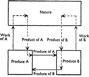
FIG. 5
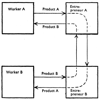
FIG. 6a
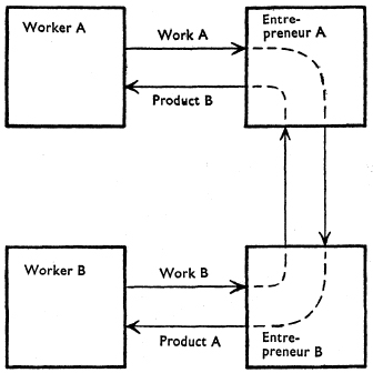
FIG. 6b
Each worker, as before, receives for his work the products of the other worker. (Neither model is, as yet, complicated by the existence of money; we are still in a barter economy.)
(2) The entrepreneur is furthermore the beneficiary of production cost differentials. We have assumed above (p. 12) that workers, for various reasons, produce with varying degrees of productivity. To produce the same amount of goods some need a greater, some a smaller, number of work-hours: or, what comes to the same thing, some produce greater and some smaller amounts of goods in the same time. In the real world the greater productivity of the work done is not generally due to some special quality of the worker, but of the enterprise in which he works. It is therefore not the worker but the entrepreneur who reaps the benefits of the higher productivity.
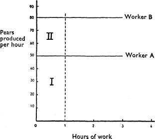
FIG. 7
Let Figure 7 represent the hourly output of two workers. Suppose worker A produces 50 pears an hour while worker B produces 80 pears in the same time. Rectangle I then represents worker A’s output per hour, that is 50 pears. Rectangle I and rectangle II together represent worker B’s output per hour, that is 80 pears. If it were the difference in the workers’ efficiency which leads to the differential of 30 pears, the wage of worker A would have to be 50 pears, and that of worker B 80 pears.
But if not worker B but the enterprise B in which he works is responsible for the higher output per hour, the owner of this enterprise, entrepreneur B, has no reason to pay his workers more than they would produce and receive if they were working in an enterprise of lower productivity—say in enterprise A, where 50 pears are produced in an hour. The surplus hourly production of 30 pears, represented in our graph by rectangle II, entrepreneur B will keep as a reward for the greater productivity of his enterprise. All workers receive a uniform wage of 50 pears, regardless of the productivity of the enterprise by which they are employed. This is what actually happens in reality. Uniform wage rates are, in principle, paid for the same work.
(3) We have defined profits as income that accrues to some individuals because others do not receive the whole output of their work in special circumstances of a temporary nature. The entrepreneur who keeps as income for himself the additional output of his workers which is due to the higher productivity, not of the workers but of his enterprise, is the profit-maker par excellence.
(4) The entrepreneur, however, is also the profit destroyer par excellence. If entrepreneur A sees that entrepreneur B can produce pears at lower cost than he can, he will try—and in the long run he will generally succeed in the attempt—to imitate his competitor’s methods of production. As a result entrepreneur A, too, will be able to produce 80 pears an hour. The output curve of enterprise A in Figure 7 will rise to the level of enterprise B. Entrepreneur A, too, will make a profit.
This, however, will not be the end of the story. Under the assumption of free competition A, as well as B, will begin to bid up wages so as to attract workers because any increase in production would enlarge their total profits. The competition for workers will clearly go on until profits are swallowed up by wage increases. Workers will then receive not 50 pears an hour but their whole output, 80 pears an hour. The whole hourly product of labor (rectangle I plus rectangle II) will be paid out as wages. This situation will change only if and when some entrepreneurs succeed in raising the productivity of their enterprises once more.
In a stationary economy, a theoretical model of an economy which goes on each day as it did before, by definition productivity does not change. There can, therefore, be no entrepreneurial profits.
Money
Entrepreneur A can obviously exchange his apples with entrepreneur B, who produces pears, only if he himself needs pears for himself or his workers. If A should prefer butter, he cannot exchange his apples with B because B has produced no butter. Butter may have been produced by C. But if B owns something which is gladly taken by others in exchange for their products, then A can sell his apples to B against this medium and use it in an exchange with C for butter. Nowadays money, mainly paper money, serves as such a medium that is gladly taken by all members of the community in exchange for their products. Money is, therefore, the general medium of exchange.
The chief function of money is to enlarge the number of people between whom exchanges can take place. It is an enlarger of exchange possibilities. It enables any one member of the community to dispose of his goods to any other member, regardless of whether the latter produces anything the first wants; the money received enables him to get the equivalent in goods he wants from a third person.
We have seen above (p. 14) how division of labor increases the productivity of the work done. Division of labor in its turn depends upon the possibility to exchange. Even if B can produce pears at lower cost, this is of no benefit to A so long as B is not prepared to take A’s apples in exchange for his pears. It follows that the introduction of money as an enlarger of exchange possibilities must result in increased division of labor and thus in higher output. Since higher output as a rule increases the amount of hours worked, the introduction of money raises living standards in two ways.
Money works not only as an enlarger of exchange possibilities, but also as an exchange act saver. Before the introduction of money apples wandered from entrepreneur A to entrepreneur
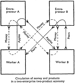
FIG. 8
B, who delivered them to his workers, while pears wandered from B to A, who delivered them to his workers—four exchange acts. Now the workers no longer receive the finished goods from their own entrepreneur, who is eliminated as a middleman between them and other entrepreneurs. With the money received from his entrepreneur each worker buys directly from other entrepreneurs—two exchange acts are eliminated.
Figure 8 shows, in very simplified form, the circulation of money in the case of apple production by worker A and pear production by worker B.
Besides being an enlarger of exchange possibilities and an exchange act saver, money has many other important functions. We shall here mention only one of them—that of an indicator of profits, as we can call it.
As we have already seen, there are no profits of the national economy as a whole. In a money economy this is even more obvious than in a barter economy. The same amount of money the entrepreneurs spend on the factors of production—the workers—comes back to them in exchange for their products. Taken as a whole, money received can neither exceed nor be short of money spent—at least so long as the flow of money is not interrupted. This latter assumption applies, by definition, to a stationary economy.
On the other hand, money is clearly the medium in which the private profits of individuals materialize. If an entrepreneur—as described earlier—can manage by his special knowledge and skill to produce 80 pears in one work-hour, instead of 50 as other entrepreneurs do, he spends 371/2 per cent less for the production of the same number of pears. The difference will show up as a stock of money not needed for the payment of wages and available for other expenditure. This is the kind of profit we have discussed above; the entrepreneur pays his workers less than the full yield of their work because this yield would be smaller if they worked in another enterprise.
Money is, however, also the indicator of another kind of private profit. It can happen that an entrepreneur makes a profit not, so to speak, at the expense of his workers but at the expense of other entrepreneurs. Entrepreneur A may receive more for his products than corresponds to his input, whereas entrepreneur B receives less. This can obviously not happen in the long run because no entrepreneur will continue spending money on production that he knows he will not get back. But in the short run it might turn out, owing perhaps to a change in tastes, that the consumer-workers spend more money on apples and less on pears than anticipated. The result will be that at the end of the production period the distribution of money among the entrepreneurs will be different from what it was at the beginning. A’s stock of money will have grown by the amount that B’s has become smaller.
We may, in this connection, add a remark on balance sheets and income statements. These show only the relative prosperity of individual economic subjects, i.e. the extent to which the income and wealth of some entrepreneurs have changed in relation to those of others. They give no information on the absolute wealth of the community because they do not indicate what can be bought with the money amounts shown. A scarcity of goods may lead to fancy prices and hence to higher incomes and capital appreciation for some entrepreneurs. This does not mean that the community’s real income or wealth has increased. A community will, on the other hand, have become richer if two-horse carriages have been replaced by 100-horse-power automobiles produced with the same labor effort. But such things cannot be gathered from balance sheets. Simple addition of the balance sheets or income statements of all the members of a community does not, therefore, tell us anything about its real product or income. This should be remembered in appraising some of the usual national income calculations.
The Time Element
Production does not go on in a timeless world. The product is not ready for consumption at the same moment as labor is expended on it. Production takes time.
From this elementary technical fact it follows that the workers cannot consume the products of present labor, but only those of previous labor. In a money economy, the money which the workers receive from their entrepreneurs in wages and spend for their living during any given production period does not buy the products of this same period but those of an earlier period. And by the sale of these products of an earlier period the entrepreneurs receive back the money spent in that earlier period.
All this is unimportant in a stationary economy, where by definition outlays and production do not change from one period to another. But in the real world there are constant changes. Only a model clearly showing the time sequence of events is useful in analysis. It would not be necessary to stress this point were it not for the fact that, under the influence of Keynes’ General Theory of Employment, Interest and Money, the tendency to use so-called circular analysis, which neglects the time element, has been strengthened.
Circular analysis presupposes that the current income of workers is spent on their current output. This would mean that current production in turn is influenced by current spending. But in reality current spending meets the products of past production which can no longer be influenced by current spending. On the other hand, the fact that a changed demand meets an as yet unchanged supply does lead to price increases and declines and to many other important changes. Only the so-called sequence analysis, as developed especially by Swedish economists, can give a satisfactory picture of these changes. For the analysis of equilibrium situations, for which they are meant in the first place, circular analyses remain permissible but dangerous because they serve very often, consciously or unconsciously, to analyze changes from one equilibrium situation to the other.
As production takes time, and we cannot therefore live from hand to mouth, a certain amount of goods in various stages of production must always be simultaneously present in the economy. Goods ready for consumption are, in the first place, essential for production by enabling the workers to survive during the production period; the other goods, as we shall see later, are essential by enabling the workers to be more productive. We shall call the total stock of these goods the capital of the community, and the individual goods capital goods.
The capital of the community is owned by people commonly called capitalists. For the time being we shall take the ownership situation as historically given. Later we shall inquire into the reasons for capital accumulation and changes in ownership.
In a money economy capitalists do not as a rule actually own the stock of capital goods. They own money and lend it to entrepreneurs, who use the money to pay their workers—who in turn use it to buy goods of a past production period.
As production goes on, new, half finished and finished goods accumulate in the hands of the entrepreneurs. Juridically these goods belong to the entrepreneurs, but economically they belong to the money capitalists because the money used for the production is owned by them. The entrepreneurs are, as it were, the trustees of the money capitalists.
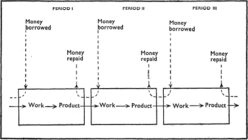
FIG. 9
When the entrepreneurs of the past period sell their products to the workers of the present period, the money they receive enables them to repay their loans and thus to free themselves from their debts to the capitalists.
Figure 9 shows how the money borrowed by an entrepreneur in the current production period is used by his workers to buy the goods produced in a past period, thereby enabling past debts to be repaid.
Expansion of Production Dependent on Capital Accumulation?
Capital is needed to keep the workers alive during the production period. We are therefore faced with the question: to what extent does any increase in employment actually depend upon an increase in capital? We shall deal with this question later in detail. Here we merely wish to make a brief remark on the so-called wage fund theory, which is the classics’ answer to this question. This theory assumed that more workers could only be employed if a store of means of subsistence had been accumulated previously by production and abstinence.
This problem—like so many others in economics—is not a real one. The present does not live at all on a store of goods accumulated in the past. The present lives as a rule on goods that flow uninterruptedly from past production into present consumption; stores of goods are neither necessary nor would they be sufficient to enable new workers to be employed. Nor is an increase of production in the past a necessary condition for an increase of the labor force in the present.
What enables an increased labor force to be employed and production to expand is the fact that the entrepreneur obtains money with which to pay new workers. This money may be borrowed from other people who have not consumed all the goods which they were entitled to receive, but have saved some of their income. But even if there are no new savings, employment and production can increase. It is not at all necessary to think of such a thing as a fixed wage fund, as the wage fund theory in its monetary form supposes. The necessary capital can be supplied through savings in other capital needs, or money can simply be created by money-issuing banks, as we shall see in Part III when discussing inflation. Finally, increased employment may not require more capital at all if there is a proportionate fall in wages.
We shall discuss the supply of capital later in detail. Here it suffices to state that neither monetary nor real scarcities need prevent an increase in employment. In whatever way the money with which to pay new workers is made available, its expenditure for labor by the entrepreneurs enforces a redistribution of past products in such a way that the new workers can survive during the current production period.
Amount of Capital Dependent on Volume of Production?
We must sharply distinguish between the question: is the volume of production dependent upon capital accumulation; and the reverse question: is the amount of capital dependent on the volume of production? The latter question is, of course, to be answered in the affirmative. If more is produced, other things being equal, there is an increase in the amount of capital, i.e. in the amount of goods simultaneously present in the economy—or, better, of goods which reach the future from the present. Such an increase in capital is often spoken of as an increase in the width of the capital structure—just as a river bed becomes wider when the inflow of water increases.
The flow of goods over time has indeed often been compared with the flow of water in a river. It is a useful comparison, and we shall use it to explain many problems in connection with capital.
Amount of Capital and Roundabout Ways of Production
Increase in production is not the only thing which causes the quantity of goods simultaneously present in an economy, the capital of the economy, to increase.
Capital can also increase when production methods become more capitalistic, more roundabout. We can illustrate our argument by returning to our comparison of the flow of goods over time with the flow of water in a river bed. If the river bed becomes wider it can contain more water than before. But the same happens also if the length of two successive river beds increases. The two streams will then overlap, as it were; the first will still be flowing when the second emerges. More water will be present simultaneously. In the same way, the goods simultaneously present in an economy must increase if production takes more time. Figure 10 illustrates this. If production takes twice as long as before, the goods previously ready for consumption at the end of Period I will now not be consumed until the end of Period II, and will therefore still be present in the economy during Period II when a new production process has already started.
The classical roundabout method of production is production by machines: a worker no longer works by hand or with a few tools, but with the help of a machine.
When a worker changes over to machine production, a new factor of production appears to have been introduced. This, however, is not the case. In the first place the machine itself consists of labor—in so far as it does not consist of raw material, which we disregard for the moment. In the second place, the machine does not really transform the worker’s work. What happens is that his present work is added to the work already incorporated in the machine.
The labor incorporated in the machine differs, however, from the labor added in the current production period in that it is work done long before the current period, and that its result is normally not consumed during the immediately following production period but in a later one. On the average, the machine remains in the production process much longer. It is consumed only over long periods. During these periods the labor incorporated in the machines, together with the labor added in running the machines, goes over into the finished goods. Even if the worker can thus produce more quickly with the help of the machine than he could without it the entire production process lasts much longer. It starts not with the current work of the worker using the machine but with the production of the machine itself, and it ends not with the goods completed currently with the help of the machine but with the last goods which the machine is still able to turn out. Only when the machine ceases to be usable at all has the last of the original labor incorporated in it gone over into finished products. This is why production with more capital, with a strengthened—or, as is sometimes said, a deepened—capital structure, takes more time.
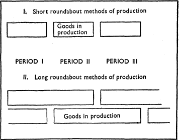
FIG. 10
How does an economy change from a less into a more capitalistic one; how does its capital structure deepen? If all the money the entrepreneurs borrow is spent by their workers on consumer goods there is, on our assumptions about their replacement needs, obviously no possibility for entrepreneurs to buy machines. But suppose the workers, or other factors of production who would in the ordinary course of events spend their income on consumption, decide to save and to put the savings at the disposal of the entrepreneurs: then the entrepreneurs would be able to buy capital goods with the money otherwise spent on consumption.
Once the economy has changed over to roundabout methods of production, no further additional saving is needed for their maintenance. The capital structure is deepened once and for all. For the finished goods into which the capital goods are ultimately converted are sold against money. And with this money the entrepreneurs are again able to repay their debts to the capitalists, who can then lend it to them again without recourse to new savings. Figure 11 shows this flow of money.
Needless to say, different goods require production detours of entirely different lengths. Productions taking detours of quite different lengths are therefore always present in an economy. The production detour of domestic help is very short. For the building of houses and skyscrapers the production detour is very long. But if the capital structure is deepened, every production detour lengthens, although not in the same proportion. The new vacuum cleaner used by domestic help, too, means a longer production detour.
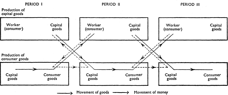
FIG. 11
The deepening of the capital structure, the lengthening of production detours, lead to increased production not by the employment of more workers but by an increase in the productivity of the single worker. Work spent on building and then on using a machine yields technically higher results than work applied immediately to the production of the end product. It is more productive.
But the reason for this increased productivity is not that the services of a machine are essentially different from those of a worker. If the machines really performed different work, if they were a different factor of production, it would be impossible for the price of machines to coincide in the long run, as it does, with their cost price. They would sell at a premium. The reason for the increased productivity is that the results of the work embedded in the machine need be available for consumption only after a longer period, that production—or consumption—is allowed to take more time. This “being allowed to take more time” is really the second factor of production, capital—if labor is considered the first.
The entrepreneur who works with machines can repay the money he borrowed from capitalists for the purpose of production only after the amortization of the machines. Per unit of product he thus needs more credits than before the extension of production detours (cf. Figures 10 and 11). For the right to use credits, and thereby to be allowed to take more time—and not for the individual capital good—he has to pay a certain compensation calculated in percentage of the amount of the credits and according to their duration. It is called interest.
What is a Stationary Economy?
This whole first part of our exposition is concerned with the working of a stationary economy. It may be useful to say a few words here on the meaning of this term, in order that the reader may follow the subsequent discussions.
When we speak of a stationary economy, we do not mean an economy in which production and consumption come to a stop. In a stationary economy production and consumption always repeat themselves in the same manner because there are no forces at work which could change them. It is an economy whose course is always exactly repeated. Such an economy does not exist in reality. But it is important to examine how such a fictitious economy would work, so as to be better able to analyze the effects of changes in important data.
The stationary economy is also often referred to as an economy in equilibrium, meaning an economy which has adjusted itself to all past and is not exposed to any further changes.
Production Exchange and Consumption Exchange
We began our economic analysis with the examination of the extremely simplified model of an economy of one isolated worker-producer. Here one single exchange act took place. The worker supplied his work to nature against products and nature demanded his work for them. We have since introduced three important features into this simple world: the entrepreneur, money and the time element.
Through their introduction the single-exchange economy is essentially changed. It becomes a two-exchange economy. Here exchange for production and for consumption are separated into two acts. The worker supplies his work no longer to nature for her products, but to the entrepreneur who demands the work against money. In a second exchange, some time later, the entrepreneur supplies the finished product to the worker who demands it against money. Money thereby serves as a sort of general representative of utility. Both the workers and the entrepreneurs value money according to the utility of the goods and services it buys on the market at current prices.
The separation of the production exchange from the consumption exchange does not, however, change the fundamental fact that in a stationary economy production and consumption are always equal. During every production period all factors of production together consume what they produce, or rather what they have produced in the past production period. And during every period the factors of production produce what they consume, or rather what they are going to consume in the subsequent period.
The Fundamental Problems of Economics
The fundamental problems with which economics is concerned can be summarized in two sets of questions. First, what goods and how many of them are produced; by what methods and by whom are they produced? And second, what goods and how many of them are consumed; by what methods and by whom are they consumed?
In a capitalist and competitive economy production and consumption are dependent on each other. Production creates income for the factors of production, and the spending of this income leads to consumption. The size and distribution of income of individuals as well as of whole groups depend on the size of total production, on what each contributes to production, and on the remuneration for this contribution. Consumption, in its turn, depends on the size and distribution of income from production. Production again depends on consumption, because the consumer by his demand determines what is to be produced. Production influences consumption, and consumption influences production.
The fact that the elements of the system are interdependent does not, however, make the system undetermined. Given certain supply schedules for the factors of production and certain demand schedules for finished products, the quantity and nature of the goods to be produced and consumed are perfectly determined. A logical chain leads from production to consumption and back. To determine the beginning of that chain is just as impossible as to establish the priority of the chicken or the egg. Every phase presupposes a preceding phase—which, however, can only be described subsequently. Since a beginning has to be made with some link of the chain, we shall for convenience sake begin by describing the production exchange. We shall inquire first what and how much is produced, by whom and by what methods production is carried on, and how the factors of production are remunerated.
Production Exchange: Production by Labor Alone
If goods were produced by labor alone there would be no problems of capitalist methods of production or of income distribution among groups of different factors of production, particularly between labor and capitalists. There would be only the problem of what and how much is produced. This problem depends, of course, on what the factors of production wish to consume, or better on how they wish to distribute their income on the purchase of various goods. But this is a problem of consumption with which we shall deal later.
Here we have only to state how much, in terms of work-hours, will be produced. The question is easily answered according to what we have already explained above. If labor were the only factor of production, work would be put into production up to the point where the money received for the work is no longer considered equivalent to the sacrifice of leisure. Money is valued here, we must remember, not for its own utility but for the utility of the goods that can be bought with it on the market according to the prevailing prices. Thus more work will be done, and production will increase either when higher rewards are offered for work—for instance, when the productivity of labor has risen—or when the workers are prepared to accept lower wages. We shall discuss this later in more detail. Here we shall but briefly anticipate: in a simple diagram like that of Figure 1 or 4 higher wage offers would mean an upward shift in the demand curve for labor, whereas willingness to work for less money would be expressed by a downward shift in the labor supply curve. It will readily be seen that both movements would result in an increase of the volume of production.
Hourly wages, i.e. the remuneration per work-hour, will—in case of a downward shift of the labor supply curve—remain unchanged so long as the demand curve for labor is horizontal. But as soon as other factors contribute to production, the demand curve for labor (for reasons to be discussed later) will run down to the right, indicating that entrepreneurs are prepared to employ additional labor only at lower wages. In this case—we shall return to it later—a lowering of the labor supply curve leads to a fall in wages. At the same time, as we shall see, the income accruing to other factors of production increases. The individual worker receives a smaller share of the community’s whole cake. But the whole cake has grown because more bakers are at work, which in turn is due to the fact that the individual bakers are content with smaller slices of cake. The total amount of cake received by all the bakers now employed, however, and even their share of it, will have become larger.
We are thus led to the important conclusion that, given an unchanged demand situation, a reduction in the individual worker’s share in the result of production is accompanied by an increase of the total product, whereas an increase in his share would entail a reduction of the total product—except under quite unrealistic assumptions concerning the elasticity of demand for labor and the elasticity of supply of other production factors.
We shall see again and again the working of this peculiar law, according to which changes in the remuneration of one factor of production lead to opposite changes in the volume of the total product.
We shall examine later on, in Part III, whether changes in wages can in certain special conditions influence the aggregate demand for goods, and whether, for instance, wage increases need not have the expected production-curtailing effects. Notwithstanding the possibility of influencing the volume of production by influencing demand, the fundamental fact remains that wage increases curtail production. This is a fact often overlooked nowadays by those who overrate the possible secondary effects of wage changes.
There is in a money economy a certain difficulty not existing in a pure barter economy: an increased product cannot be exchanged through the medium of the same amount of money unless the price level declines. We shall, for the time being, evade this difficulty by assuming that enough new money is always introduced into the system to prevent a decline in the price level. The price stability so ensured does not, however, imply wage stability. If labor becomes more modest in its wage demands, the wage level falls relative to the price level. The difference between the amount of money spent on wages and the amount of money received from sales accrues to other factors of production as income.
Production by Labor and Capital
Goods are not in the real world produced by labor alone. Capital is another factor of production. We have described above the nature and significance of capital. Production can require more or less capital. Even in the most primitive circumstances some capital is needed for the survival of the workers during the production period. Modern production, with its very roundabout methods, needs much more capital. As production detours lengthen—say double—a double amount of capital must be in the hands of entrepreneurs. In a modern economy work is directed into roundabout methods of production by entrepreneurs, who borrow money in the form of credits from banks or in various forms from other money owners and spend that money on capital goods. If entrepreneurs should wish to double the length of the production detours, they would need to borrow a double amount of investable funds. The length of production detours depends, therefore, on the supply of and demand for investable funds.
Investable funds are directly or indirectly supplied by people who save money instead of spending it on consumption. How large is the supply of investable funds by savers? In a stationary economy, where changes are excluded by definition, we have to ask: how large is the total stock of savings? We do not ask how large is any addition to the stock by new saving. New savings are not necessary to uphold the status quo of production detours. The money received from the sale of finished products enables the entrepreneurs always again to acquire the capital goods or semi-finished products they need.
The amount of saving offered is, like every supply in a free economy, a function of the price, i.e. the interest rate. The question of how the supply curve for savings runs in general is controversial. Some people deny that the supply curve runs in the usual way upward to the right, which would indicate that more is saved and more savings offered at a higher interest rate. These authors assume that the curve runs vertically, meaning that the amount of savings is independent of the interest rate. This may or may not be the case. The important point here is that the curve never runs horizontally, i.e. that the supply is never unlimited.
Note that we are here dealing with the question of how much will be saved out of a given income. The further question, how changes in income call forth changes in savings, will be treated later when dealing with the changing economy. The latter question should never detract attention from the former.
What, on the other hand, will be the shape and level of the demand curve for credits, i.e. how much capital will be demanded at the various interest rates? In other words, how much interest will the entrepreneurs be prepared to pay for various amounts of capital?
Capital increases the productivity of the labor used in production. Suppose the length of detours of x years of a production in which y dollars are simultaneously invested is increased by 10 per cent of x years. They then obviously need simultaneously 110 per cent of y credits. Suppose that by such an increase of length the annual product increases by an amount equivalent to the output of three workers. Then, obviously, the entrepreneurs would be prepared to pay for the additional credit necessary an interest sum pro anno corresponding to the wages of three workers. If the next extension of production detours would again increase the product by the same amount, the entrepreneurs would again be prepared to pay interest corresponding to the wages of three workers. The demand curve would run horizontally. For every additional new quantity of capital the same interest would be offered.
But in reality every additional quantity of capital is less valuable than the former. Therefore the demand curve for credits does not run horizontally but downward to the right. So if the supply of capital increases, the interest rate must decline.
The Law of Diminishing Marginal Returns
This is due to the so-called law of diminishing marginal returns, with which we have to get acquainted now. It is a technical law. It is concerned with the technical productivity of one factor of production used in combination with another.
The law states that, given a certain amount of one factor—labor for instance—the addition of every further unit of the other factor—e.g. capital—increases the productivity of the first factor, but in a decreasing degree. The validity of this law will readily be understood if we consider that an amount of capital applied to labor, for instance in the form of a hammer, is likely to raise the productivity of labor much more than the same amount of capital used for the last refinement of a capitalistic process. This law of diminishing returns, or better diminishing marginal returns, means that the entrepreneurs will be able to pay less interest for every additional amount of capital.
We can now establish how much capital will be used in our stationary economy. Just as on every other market, the quantities borrowed and lent on the credit markets are determined by the intersection point of the demand and the supply curves. Capital will be saved and employed in production up to the point where the higher interest demanded for additional credits can no longer be paid by the entrepreneurs because the additional amounts of capital no longer increase productivity to a corresponding degree. The lending price for capital, the interest rate, is determined by the marginal supply of and the marginal demand for credits.
It should be noted in this connection that the question of combination of capital and labor is not identical with the question of the optimum size of the plant. Nor should either question be confused with the question of the optimum combination of so-called fixed and variable capital. These questions will be treated later on. They do not exist in a stationary economy, where we must assume that adjustments to the optimum size of plants and to the optimum combination of fixed and variable capital have already taken place.
Production Factors are Remunerated according to their Marginal Utility
It is sometimes said that the distribution of the proceeds of production takes place according to the contribution of the factors of production to the total product. Labor receives what is to be imputed to labor; the capitalist receives what is to be imputed to capital. But this is an antiquated and over-simplified way of expression. In reality, the worker, equipped with a certain amount of capital, produces a certain amount of goods—no doubt more than he would have produced without capital equipment. But once labor is so equipped, it is impossible to find out how much of the product is to be imputed to labor and how much to capital. The product is just the result of productive labor. The only thing which can be discovered is how much the product has increased by the addition of the last unit of capital. We can calculate the so-called marginal productivity of capital.
The marginal productivity of capital determines not only the amount of capital used at a given supply of capital; it also determines what part of the total product is branched off and accrues to the capitalists in the form of interest payments. This part is by no means equivalent to the total amount by which production has increased owing to the use of capital. It is less because in accordance with the law of diminishing returns the marginal productivity of capital is less than its intra-marginal productivity. The benefits of the intra-marginal productivity of capital accrue to the workers in the form of higher wages. They cannot be distinguished from the productivity of labor as such.
Production with Land
In addition to labor and capital there is allegedly a third factor of production—land. The production factor labor is always used in conjunction with or on the production factor land. Only the combination of labor and land—plus capital which draws production into detours—leads to the production of goods.
Land is needed in agriculture because we can sow and reap harvests only on land. Land is also necessary for every other production. The workers have to work somewhere. They cannot work in the clouds.
Economics is usually concerned only with agricultural land or urban landed property. But coal or oil fields are also land. There is no difference of principle between land yielding wheat and land yielding coal, or a river used for navigation or water power. We shall treat as land every part of the surface of our earth that yields space and natural resources, such as coal, minerals and so on. The sea, too, can be considered land in this sense.
Land was formerly defined as the eternal and indestructible basis of all production. This is too narrow and even a wrong definition. If the soil is not conserved, it gets exhausted as do oil wells and coal mines.
As a site for production and consumption land indeed renders eternal services. Its utility to man can, however, vary within wide limits. It can increase, for instance, by the introduction of new means of communication.
The utility of land is identical with the utility of all services rendered by it. If these services are limited, in time the value of land is generally considered as the sum of all these services. In so far as the services are eternal, land is valued as the carrier of recurring annual yields. As we shall presently see, the price of land is equal to the money value of these annuities, capitalized at the prevailing interest rate.
Is Land a Third Production Factor?
It is customary to speak of land and of the products of nature as a third factor of production besides labor and capital. It is equally customary to assume that land and its services can generally be rented for “rent”—as capital is borrowed for interest.
This approach is unrealistic and leads to analytical difficulties. It cannot be denied that land, such as coal and oil fields, is often rented for use or exploitation. Machines, too, are sometimes rented. However, it is far more general for entrepreneurs to buy and not to rent the land where they intend to build their plant, just as they buy their machines rather than hire them.
If we treat land in principle as being rented rather than bought, then we neglect in our analysis the fact that land has to be carried through time just as other capital goods, that it takes credits to do so and that, therefore, an entrepreneur buying land with borrowed money thereby influences interest rates.
Entrepreneurs themselves make no distinction of principle between buying labor, machines or land. Their calculations distinguish only between two totally different kinds of costs: on the one hand the annually recurring interest they pay for the money they borrow, and on the other hand the prices they pay, once only, for labor, capital goods or land bought with the borrowed money. There is for an entrepreneur no difference between a machine in his plant and the land of the site of his plant, just as there is no difference of principle between labor and machines. Machines are labor of previous production periods. Nor can in many cases the land component be distinguished in practice from the labor component.
We shall thus treat land as a sort of capital good, provided by nature rather than by man. We shall consider only two factors of production: first labor, including land as a carrier of services, for which the entrepreneur has to pay a price; and second money capital or credit, for which he has to pay interest.
The Price of the Services of Land
There remains, of course, the question of the pricing of land. Its price will obviously depend on the services land offers to entrepreneurs, including in particular agricultural entrepreneurs, i.e. farmers—just as in a slave society the price of a slave would depend on his services. In a society of free men, of course, only the services have a price and not the man who renders them.
Land, just as capital, is useful to the entrepreneur because it replaces work. This seems paradoxical at first sight, for in raising a crop land does not merely replace labor but is indispensable. It can never be replaced even by the greatest number of workmen. But the absolute absence of land is a limiting case that can be neglected for analytical purposes.
Given a certain area of land and certain amounts of labor, every addition of land for cultivation will increase the productivity of the existing workers and thus replace workers, just as every additional worker will increase the productivity of the existing land and thus replace land.
However, here too we meet the law of diminishing returns, as in the case of the productivity of capital discussed above (p. 40). The productivity of a given number of workers cultivating land of a given quality will increase with the addition of more and more acres, though in a decreasing degree.
Entrepreneurs will obviously be prepared to bid for the service of every additional unit of land an amount as high as the wages of the workers that the addition of this unit can replace. Given a certain supply curve of land services the price of the service is herewith determined.
Land serves not only production but consumption too. A nation’s most important durable consumer good is its housing stock. Houses cannot be built on air—they have to be built on land. The value of urban landed property depends on how much of their income consumers are willing to spend for living in certain districts. In essence the problems involved are the same as those we have been discussing earlier in connection with the choice between the consumption of apples and pears.
The Price of Land
In the real world entrepreneurs do not buy the services of land as they do the services of workers. They either rent or buy the land as a carrier of services. It is the usefulness of the services which determines the rent as well as the purchase price of land. The rent for a certain period, say one year, is equal to the value of all the services the land renders during the year. The latter, too, are called rent. But what are the principles which determine the price of land to be bought? One would expect the price of land to be equivalent to the sum of the prices of all the services it renders. But the following has to be considered.
In so far as the services of land are perpetual, the price of land would obviously have to be infinitely high, were it not for the fact that the purchase price is paid in money and that money if lent as credit also yields a perpetual service, namely the interest the lender goes on receiving. Thus the price of land must stabilize at the point where the interest on the purchase price is equal to the price of the service the land renders during a certain period. In other words the price of land is, in principle, the price of its service capitalized at the long-term interest rate for credits. If the service is worth $5 a year, and the interest rate is 3 per cent, then the price of the land is $166, for 5/x = 3/100, therefore x=500/3=166.
If the services of the land—of a coal field for instance—are not perpetual but last only, say, 10 years, the calculation is somewhat more complicated. In this case it is not possible to compare the rent with the interest payments because only the latter are perpetual. One has to compare the present utility of the money on the one hand and that of the annual services of the land on the other. The money is, of course, worth its face value. But if a unit of land annually yields $5 for 10 years, it is worth not 5 x 10, or $50, but less. Since present money yields interest as of today, whereas the annuities yield interest only as of their payment, the annuities can only be valued at a so-called discount. At an interest rate of 3 per cent, land yielding $5 during 10 years and nothing thereafter would be worth about $43.
It may be asked: why is the price of land equal to the capitalization of the services it yields, whereas machines sell at production cost? The answer is that machines can never cost more than their production costs, for their number can be increased at will by payment of these costs. Nor can the productivity advantages of a machine ever be greater than the interest on the cost price calculated for the lifetime of the machine. If the advantages were greater than this amount of interest ever new machines would be constructed. Land, on the other hand, is produced by nature once and for all. It is scarce and cannot be increased by work. Its services are fixed and are not influenced either by production costs or rates of interest. But since in the long run money lent as credit and money invested in land must offer the same yield, the price of land must stabilize at a level where the interest on the purchase price equals the price of the services. Changes in the interest rate must, therefore, entail inverse changes in the price of land. A falling interest rate raises land prices and vice versa.
Differential Rents and Differential Prices
Land is not homogeneous, as we have assumed so far. It differs in quality. One of the chief qualitative differences of land rendering comparable services in other respects is the result of differences in distance from production and consumption centers.
Suppose the last additional unit of what we could call standard land, cultivated by 1,000 workers, increases the productivity of those thousand workers by the product of five workers. There may exist other land of which the last unit, added to an equal area, increases the productivity of the same number of workers by the product of three, two or one worker. There may even exist land of such poor quality that additional amounts do not increase the product at all—marginal land.
Except for this last-mentioned case, entrepreneurs will be prepared to pay money for all land, but obviously less than for standard land. Their bids for various sorts of land will vary according to the work-replacing capacity of the land. Land of which additional quantities add nothing to the productivity of a given number of workers is worthless and generally free, i.e. it is nobody’s property.
The classical economists explained all the advantages accruing to the owner of land—they called them rent or ground rent—by the fact that good land yields more than bad land. In a certain sense all ground rent is indeed differential rent. But in this sense all wages, too, are differential rents. They are the difference between what is paid to a worker of high and to a worker of low or zero productivity. But the differential rent theory does not explain the laws according to which land of a given quality cultivated by a given number of workers is to be valued. Nor does this theory explain the point at which land becomes marginal.
The expression rent, and more particularly ground rent, for all the benefits land yields to its owners is none the less still in current use.
Obviously land of very different quality is used simultaneously, but as land of lower quality yields less vast acreages of it are equivalent to small areas of good land.
Differential rents and differential prices caused by quality differences should not be confused with the rents and prices of homogeneous land of a certain quality worked by a given number of workers.
Homogeneous land of a certain quality yields its owner a revenue which corresponds to the additional productivity of the last unit of such land taken into use. The benefit of the higher productivity of preceding units accrues to the workers in the form of wages.
Land of inferior quality yields less revenue according to its lower productivity. Compared with the rent of such inferior land the rent of the better land is indeed a differential rent.
Rent from good land can never be higher than rent from inferior land offered at correspondingly lower prices. Scarcity of land is a relative concept. With correspondingly higher demand inferior or more distant land is taken into use. The “frontier” moves further out.
Land Prices, Wages and Interest Rates
We have so far examined what determines the value of the services of land and its price on the assumption that the number of workers and the amount of investable funds are given. In reality neither is ever given; both are subject to constant change.
We shall examine the effects of changes in the supply of and the demand for capital and labor later on. Here, only a few preliminary remarks.
If the supply price of labor, i.e. the wage demands, declines, more workers can be employed, as explained earlier. Given a certain amount of land, each worker will then have less land to work on. The law of diminishing returns works in the opposite direction. The productivity, i.e. the labor-replacing capacity of the land, becomes greater. The rent from land increases.
If the supply price of capital, i.e. interest, declines, the cost of production declines. But the cost reductions vary according to the length of the production detours. With short production detours costs decline to a lesser degree than they do with long production detours, because capital costs enter into the former less than into the latter. Now the use of land means a long, in fact an infinitely long, production detour. If somebody borrows money to buy land, he has to pay interest on this money in eternity in order to profit from the land’s equally eternal and not amortizable benefits.
For this reason a lowering of interest rates must mean a very substantial reduction in the cost of the use of land. This reduction in costs will result in sub-marginal land becoming marginal. This land will now yield a revenue even though its technical productivity has not risen. All land prices will go up until the—now lower—interest on the—now higher—prices is again equal to the rent.
Variable and Fixed Capital
We have already mentioned that the production detours made possible through the use of capital are of different lengths. Labor used for the construction of a machine and labor used in working a machine represent the most important examples of such differences in length. In the former case the product of labor is fully consumed only when the machine is worn out; in the latter case labor—including work for the production of raw materials fed to the machine—is as a rule consumed not long after input. Capital which cannot be consumed or converted to other uses until after protracted time periods, such as machines, industrial plants and so on, is called fixed capital. Capital such as that embodied in the consumption fund for workers or in raw materials, which can quickly be consumed or easily be switched into other forms of capital, is called variable capital. There is, however, no sharp borderline between the two kinds of capital.
It is often contended that fixed and variable capital have to be combined in a certain way for technical reasons. It is assumed that a certain number of workers, a certain amount of raw material, and a certain amount of capital equipment must be combined if optimum results are to be achieved. This view, however, over-simplifies the problem.
There are really two problems involved which have to be clearly distinguished. On the one hand, there is the problem of the combination of variable and fixed capital generally, and, on the other, the combination of variable and fixed capital frozen into certain forms.
As regards the first problem we must remember that work as such can always be applied to simple and relatively inexpensive as well as to complicated and relatively expensive machinery, and that raw materials can be transformed into goods with the help of the former as well as of the latter. In other words the amount of fixed capital is never determined a priori. The use of fixed capital is determined by the same laws as is the use of capital in general. It is applied up to the point where the cost of additional fixed capital is still matched by a corresponding increase in productivity.
Now the demand for fixed capital is much more sensitive with respect to interest rates than is the demand for variable capital. Whether credits are available at 3 per cent or at 4 per cent makes hardly any difference if they are used for wage payments, but a great difference if they are used to buy real estate or to build factories. The reason is that in the first case small amounts, and in the second case large amounts, of credit are needed per unit of finished goods. It is, therefore, the height of the interest rate which, at a given marginal productivity of fixed and variable capital, determines the way in which both are combined. There is no a priori optimum combination.
The second problem, that of the optimum combination of variable and fixed capital frozen into certain forms, is a short-run problem which does not arise in a stationary economy, where by definition the length of production detours does not alter any more, and where, therefore, it is immaterial whether capital is frozen into certain forms or not.
The second problem is not concerned with the question whether workers should, for instance, work with hand tools or at one huge steam hammer. It is concerned with the question of what happens when there is a change in the combination of variable and fixed capital once the steam hammer is installed—for instance if workers are dismissed or new workers taken on. It is the combination of variable capital with certain existing capital goods rather than with fixed capital as such that is at stake.
Suppose employment is curtailed because wages have gone up or prices gone down, as the latter do in depressions. Then the entrepreneur uses less variable capital. But the use of fixed capital frozen into certain capital goods like machines, plants, etc., cannot be undone retroactively. The fixed capital and the charges payable on it remain the same even when the entrepreneur has curtailed his use of variable capital. This leads, indeed, to combinations of variable and fixed capital which cannot be optimal.
In the long run, however, there cannot be other than optimum combinations between variable and fixed capital; they are determined by the productivity of fixed capital and of variable capital respectively and by the interest rate.
The Size of the Firm
Not to be confused with the problem of the best combination of variable and fixed capital is the problem of the optimum size of the firm, that is of how many units of combinations of fixed and variable capital should be joined together physically and/or financially in one place or under one management.
In practice this is a question difficult to decide. In theory the answer is easy. There is one particular size for each firm at which its costs are lowest. If the firm is smaller, its overhead expenses per unit of product increase. If the firm is larger, bureaucratic methods, for instance, lead to the same result. The task in practice is to determine the exact size at which the cost-increasing forces are at their minimum.
In a stationary economy deviations from the optimum size of firms are excluded by definition. Here it has to be assumed that the adjustment to the best size has taken place and no more changes occur. It is only when the output of an industry suddenly increases or decreases that the size of an enterprise may turn out to be larger or smaller than optimal. Entrepreneurs continue to produce in the existing plant, rather than close down factories or build new ones.
Even if entrepreneurs manage in such cases to combine fixed and variable capital in the optimum way, they will still be faced with the difficulty that the single firm may have become too large or too small. In either case unit costs increase.
Variable and Fixed Costs. Total Costs. Unit Costs and Marginal Costs
The use of fixed and variable capital involves certain expenditures. During a production period—or as we may assume at its beginning—entrepreneurs spend money on variable capital goods, particularly raw materials and labor. These expenditures, which include also interest payments to the capitalists who lend the money so used, are called variable costs of production. Entrepreneurs furthermore have to spend money for those parts of their fixed capital goods that are being consumed during the period. (The main part of the fixed capital is carried over into the next production period as the capital stock.) These expenditures, which include also the interest payments on fixed capital, are called fixed costs. Variable and fixed costs together are called total costs of production.
The combination of fixed and variable costs is, of course, a function of the combination of fixed and variable capital. This means that in the long run there is no special problem of optimum combination of variable and fixed costs. In the short run there is such a problem: variable capital declines or increases—with declining or increasing output—whereas the fixed capital frozen in certain capital goods remains the same. Therefore variable costs fluctuate, whereas fixed costs remain more or less stable. This has certain consequences for the so-called unit costs, i.e. the total costs divided by the number of units produced.
If less is produced than anticipated when the fixed capital goods were installed, the entrepreneurs will have more machinery, land, etc., in hand than they need for the smaller output. Fixed costs do not decline as much as output. As they have to be distributed over a smaller production, unit costs increase.
If more is produced than anticipated variable costs rise—for instance because work can be organized rationally only in a factory which has been appropriately enlarged. This, too, leads to an increase in unit costs.
Unit costs will thus be lowest when production is exactly of the size which long-run plans anticipated it to be. When production is smaller the stability of fixed costs, when it is larger the increase in variable costs, will tend to give an uplift to unit costs.
All this is treated very elaborately, too elaborately perhaps, in the usual textbooks on economics. The development of unit costs is usually represented by a graph, which we reproduce in Figure 12 in a form which though greatly simplified is sufficient for the purposes of our argument. The graph shows three kinds of curve: the marginal cost curve, the unit cost curve and three price lines. The marginal cost curve indicates at what additional cost additional units can be produced. The price lines show the price the product can bring on the market. Production, as we know, expands up to the point at which the price just covers marginal costs, i.e. the cost of the last additional unit produced. The intersection points of the marginal cost curve and the price lines indicate the amounts that can be produced. In our graph the $10 price line cuts the marginal cost curve at an output of 10,000 units (P1). At a market price of $10, 10,000 units will be produced. Assuming that this is the output for which the plant has been planned, this will be the point of optimum combination of variable and fixed capital. Unit costs will be lowest at this point and will coincide with marginal costs. For any output larger or smaller than 10,000, unit costs will be higher for the reasons explained above. The unit cost curve rises to the right and left of P1. It is said to be U-shaped.
A change in price causes a shift in the point at which the costs of the last additional units are still covered. Output will change. If the price declines to $5, the price line in our graph cuts the marginal cost curve at 5,000 (P2), and output will shrink to 5,000. If the price rises to $15 per unit the marginal cost curve and the price line intersect at 15,000 (P3), and output will rise to 15,000.
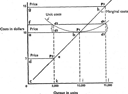
FIG. 12
What will be the effect on the entrepreneur’s profit and loss of these changes in output? For simplicity’s sake we shall assume an entrepreneur who is able to produce 10,000 units without profit or loss at a sales price of $10. His revenue, as his costs (price and unit costs multiplied by production), correspond to the area a-b-i-c. If the market price drops to $5, his output drops to 5,000 units. His revenue is reduced to an amount which corresponds to the area c-d-e-k whereas his costs are c-f-d2-k. For, due to unchanging fixed costs, his unit costs have increased by dx-d2 to k-d2. He suffers a loss which corresponds to the area d-f-d2-e, a loss which, however, can never surpass the fixed costs. For if the variable costs are no longer covered by the revenue, production will be stopped.
If the market price rises to $15 and the production to 15,000 units, the revenue of the entrepreneur rises to c-g-h-l. But because his unit costs have risen by d3-d4, his costs are now c-f-d4-l and his profits are not a-g-h-d3 but f-g-h-d4.
All this is valid not only for each individual entrepreneur but also when the general price level fluctuates, as in inflation or deflation, for the whole economy, i.e. for all the entrepreneurs together.
The Consumption Exchange
We have so far examined the production exchange, by which the factors of production supply their contributions to production in exchange for money as a sort of general representative of goods. For what goods, for how many of them and by whom, will this money be spent in the consumption exchange to which we now turn?
The first thing to note is that, provided there is no interruption in the flow of money, all the money present in the economy must be spent on all the products coming to the markets. All the money buys all the goods. As a result, a certain price level will be reached at which the supply of goods and monetary demand balance. This is the starting point of the famous so-called quantity theory of money, which deals with the relation between the quantity of circulating money and the price level. We shall return to this later in connection with inflation and deflation.
But what products will be demanded and by whom? The quantity theory does not furnish us with an answer to either question. The two questions are closely related. What goods are demanded for consumption depends essentially on the distribution of income. A wealthy capitalist will generally wish to consume other goods than a low-salaried employee. The distribution of income in turn is dependent upon the contribution to production of each of the production factors and upon their remuneration. In the long run consumption follows production just as production follows consumption.
Since the distribution of income is of paramount importance for consumption demand, we shall briefly recapitulate the following points.
(1) Labor is rewarded for its contribution to production by the payment of wages on the part of entrepreneurs.
(2) The capitalists, who lend entrepreneurs money for wage payments and the purchase of capital goods, are rewarded by the payment of interest.
(3) The share of the total product which the capitalists receive is determined by the marginal productivity of capital. For each unit of capital they receive a reward corresponding to the productivity increase due to the last unit of capital added. This reward is smaller than would correspond to the productivity increase due to intra-marginal units of capital. The difference accrues to labor in the form of higher wages.
(4) No separate allowance is made in our model for rent as a reward for the owners of land. It is assumed that land is bought in the same manner as capital goods and that its contribution to production is, therefore, rewarded by the interest paid to the capitalists who have lent the money for the purchase. To assume that the landowner receives a rent would be tantamount to counting twice the reward for the use of land. The landowner gets his reward in his capacity of capitalist. He lends the money which he receives for the sale of the land.
The Purchase of Intermediate Goods
The factors of production receiving money in the production exchange for their contributions to production spend this money in the consumption exchange for the goods of the past period in order to consume them and to survive during the current period.
This description of the process is, however, only partially correct. As we explained in connection with roundabout methods of production, entrepreneurs buy not only labor of the current period (using the machines) but also labor of past periods (building the machines). The purchase of intermediate goods is again mentioned here because in a certain way it, too, belongs to the consumption exchange category and occupies an intermediary position between production exchange and consumption exchange. Just as in the case of consumption goods the products of past labor are purchased. And again the receipts from the sales enable the sellers to continue production in a new period.
On the other hand the purchase of intermediate goods belongs to the category of the production exchange inasmuch as the products of past labor are not consumed immediately but directed into the longer production detours, so that their consumption does not take place in the current period but together with that of the labor of the current period in a later period.
Equality of Production and Consumption
The goods supplied during a production period for consumption or as intermediate and capital goods and the goods actually consumed or used as intermediate and capital goods are necessarily the same. This is a truism in a stationary economy which is, by definition, in equilibrium. In an economy in equilibrium all goods produced are also consumed, for otherwise they would not have been produced. This is the substance of a law known as J. B. Say’s Law of Markets. In a changing economy, such as it exists in reality, this law is not always valid. We shall later return in detail to the questions connected herewith.
Equality of Costs and Revenue
Input and output comparisons in real terms are either truistic—because labor produces neither more nor less than it actually produces—or nonsensical—because labor and product cannot be reduced to a common denominator. But how about comparisons between the money spent for production—the money costs of firms—and the money received for products—the money revenue of firms? The statement that money costs equal money revenue is, as such, not at all nonsensical, for sums of money can be compared with each other.
But it is again a truism to say that costs equal revenues when the costs and the revenue of the whole economy are meant. Clearly, in a stationary economy all the money spent must be recovered as revenue.
The statement that costs equal revenues for the whole economy has to be sharply distinguished from the statement that costs equal revenues for a single entrepreneur. This latter statement is no truism but, in a stationary economy, is necessarily always correct. It implies that the money spent by an entrepreneur on factors of production and the money received by him for products must balance in the long run. For a deficit would restrict, and a surplus would expand, the production of any entrepreneur until costs and revenues again balance.
Labor and goods cannot be compared for lack of a common denominator. But each entrepreneur’s contribution to the total production expenditure of an economy can be compared with his share in the total product. Since, in an economy in equilibrium, entrepreneurs’ monetary receipts exactly match their expenditure, each individual entrepreneur’s percentage share of total input equals his percentage share of total output. For the money paid by each entrepreneur to the factors of production represents a certain percentage of the total money stock of the economy and thus attracts the same percentage of productive forces into his enterprise. The money received, too, represents the same percentage of the money stock. This proves that the entrepreneur’s percentage share in the total product of the economy is the same.
In a stationary economy an entrepreneur is certain of the demand for his products and of the resulting price conditions. But in a changing world he might make mistakes because the future is uncertain. In a changing world costs and revenues might not balance in each case. The demand for pears and their price may rise, those for apples fall. The producers of apples will then receive less than they spent, the producers of pears more. Profits and losses will result.
The Profits of Entrepreneurs
We are now in a position to add some precision to our earlier remarks about entrepreneurial profits.
(1) Profits in the sense we use the word—in accordance with the definition of Schumpeter and Knight but contrary to the business man’s notion—does not include the return on the capital used and the compensation for managerial services.
(2) If profits cannot exist in a stationary economy, then they can, in a non-stationary competitive economy, only be of a transitory nature.
If, due to a change in taste, more of one product and less of another is wanted on the markets, the price of the first product will go up, the price of the second will go down. The producer of the first product will make a profit, the producer of the second a loss. But after a certain time profits as well as losses will disappear. The firm which makes a profit will expand, that making a loss will restrict production until prices and costs again reach balance through the changed supply position.
Profits may, however, be the result not only of higher prices but also of lower costs. Technical progress is one of the chief reasons for declining costs. The dynamic entrepreneur who is the first to make use of new inventions or of new methods of production makes profits. But as time goes on, other entrepreneurs follow his example. All entrepreneurs are then able, and through competition among themselves forced, to pay higher prices for the factors of production: profits disappear.
If, however, the new invention or method of production is protected against imitation by patents or secrecy, the profits remain—they become “frozen”. Monopoly profits, too, are essentially such frozen profits.
(3) Profits are not really, as often stated, a reward for bearing a risk. The entrepreneur reaps a profit not because he has taken a risk but because he has been correct in his anticipations. If he has not been correct, he suffers a loss and does not gain a profit. The profits arising from the changes are the counterpart of and not the reward for the risk.
(4) Profits can be made only by individual entrepreneurs and not by the economy as a whole.
In the case of profits through change of taste this is quite obvious. If the total amount of purchasing power in the hands of the population is limited, the prices of certain products can rise only if those of others fall.
But the statement is also correct in the case of profits through cost saving. From the point of view of the whole economy, cost savings represent increased productivity of the factors of production, particularly labor, but not profits.
Thus a sharp distinction must be made between the resulting stationary benefits and the temporary profits made by individual entrepreneurs who deprive the production factors of the benefits of the productivity increase and keep these profits for themselves. Profits are interpersonal shifts of income; they are private in character and do not concern the national economy as such.
(5) The so-called losses of the national economy through misdirection of production or through faulty investments are not losses of the national economy either. Suppose a luxury hotel is built and later goes bankrupt for lack of clients able to pay luxury prices. This does not mean that the labor spent on its construction is lost for the whole economy. The rooms may later be rented to more modest clients at reduced prices. From the standpoint of the community it does not make any difference what class of people enjoy the luxury of the hotel. What the misdirection of production has accomplished is only that the final distribution of the total product of the economy does not coincide with the initial distribution of wealth. The owners of the hotel have lost to others their claim to the products of a certain amount of work because they over-estimated the demand for the product of their investment. Misdirection of investment can lead to national losses only if entrepreneurs, through lack of further finance, have to abandon a construction project before it is able to render any services—say a half-built railway. But in such cases other entrepreneurs will usually acquire the assets cheaply through forced sale. These other entrepreneurs will complete the project. The latter may even become profitable for them since their fixed costs are much smaller. In any case the losses here, too, are private and not national ones.
(6) This economic misdirection by misjudgment of demand has to be distinguished from what could be called technical misdirection. If an entrepreneur uses methods which are inferior to those that can be used or are being used by others, the productivity of the whole economy is affected. In this case one speaks frequently of a loss to the whole economy. A lowered productivity of an economy which results in a lower aggregate output is, however, not a loss in the sense of the counterpart of a profit as defined.
Profits, Interests, Rents
Profits and interests should always be sharply distinguished from each other. The latter do not disappear through adjustment to changes. Capital is remunerated by interest payments in a stationary as well as in a changing world, at least so long as capital supply is not unlimited.
The so-called rents, too, are not in principle transitory in character. Linguistic usage is somewhat vague in these matters. What is meant by rents in the first place is the additional income accruing to certain entrepreneurs due to inventions or production methods protected by law, or due to a monopolistic position. These are the frozen profits of which we spoke earlier. Frequently rents are also understood to mean all the monetary receipts or advantages of a more or less durable character which accrue to the owners of certain property, such as land (ground rent) or claims and titles (annuities, perpetual rents from non-redeemable securities, etc.).
Rent, in the sense of what is paid for a lease, is also of durable nature. Rent in this sense is normally the money paid for the use of land, houses, certain machines, patents, or other carriers of services. This money is paid to the owners of these carriers by people who need the services for production or consumption, but who are not willing or able to buy the carriers.
The rent paid for the use of land is, in principle, always equal to the value of the services of the land. In case of divergences the land would be bought rather than rented, or vice versa. The rents for land and for all goods which are not freely reproducible lead, as it were, a separate existence of their own; they are independent of the rate of interest and of any production costs.
Things are different in the case of rent for property which, like built-up land, is partly, or like machines wholly, reproducible. These rents are dependent upon interest rates. Rent for machines must always equal the interest on their purchase or cost price. If the rent rises beyond that interest it will become profitable to build more machines for the purpose of renting them out. If the rent falls below the interest, the production of machines falls.
If interest rates fall, machines requiring a higher capital outlay can be taken into use. The productivity of those machines is greater, but the marginal productivity of the capital incorporated in them is smaller. The rent for those machines, calculated on the cost price, will fall accordingly.
The rent for plants installed previously at higher interest rates will fall even more. The owners of the old machines save less labor per unit of output than do those of the new machines, yet they have to compete with the latter for labor. The return on the old machines is smaller than the return on the new ones, and the rent for old machines falls below the rent of new ones.
If the machines are not leased but sold, then their owner incurs a corresponding loss by selling below his cost price. For the buyer of the old machines can compete with the owners of new machines only if his higher production costs are matched by a saving of interest on his purchase price.
Security Prices
We do not wish to conclude our description of the fictitious stationary economy without drawing some preliminary conclusions concerning stock price formation. In doing so we have to bear in mind that we are dealing with an economy in equilibrium: the economy is not subject to changes—in particular the demand for and supply of capital, and therefore the interest rate, are constant. This stationary economy is also a riskless one. The future is like the present, and the present of course is known to all.
In such an economy in equilibrium all loans are always worth exactly the original sum lent. No matter how long the duration of the credit, all credits are always worth “par.”
For short-term credits the above statement is obvious. So long as the debtor is solvent—and in a stationary economy he is so by definition—the claim is worth 100 per cent.
Capital is made available to entrepreneurs mainly against common shares, preferred shares or bonds. Such capital does not become due for repayment for long periods, or indeed at all.
In a stationary economy the price of common shares would always equal the original issue price. Dividends would equal interest on the issue price at the prevailing interest rate. Entrepreneurs would be able and willing to pay in dividends on the shares exactly as much as they would have had to pay in interest for a loan equalling the issue price of the shares. At an interest rate of 5 per cent dividends of $5 would be paid on each share issued at $100. The share would always be worth exactly $100.
For preferred shares bearing fixed dividends and for fixed-interest bonds the proposition is even more obvious. They would always be worth par provided the preferred dividends and interests are fixed in accordance with the prevailing interest rate, as they must be in a riskless economy in equilibrium.
The fact that long-term investments are worth par and that their yields, i.e. their interest payments as a percentage of their price, are always equal to the interest rate paid for credits, is important for the understanding of the price formation of securities. Naturally, significant qualifications have to be made in the real, changing and uncertain world. We may anticipate two essential points.
(1) There is always a risk that the expected earnings might not materialize, and even that losses will be incurred. If the risk is considered high, a common share paying a dividend of $5, at an interest rate of 5 per cent, might not be worth $100 but only $50 and thus yield 10 per cent.
(2) There is always a risk of future changes in the interest rate. If people are “bearish” regarding the interest rate, i.e. fear that it will fall, then the price of long-term investments will be above par and their yield below the prevailing short-term interest rate. On the other hand, the price of long-term investments may be lower than par and their yield above the prevailing short-term interest rate if people are “bullish” regarding the interest rate, i.e. expect it to rise. While both cases happen in practice, the latter seems to be more frequent. Long-term investments as a rule yield a higher return than short-term investments. This proves that generally debtors fear and creditors hope that funding operations, i.e. transformation of short-term into long-term investments, will in future only be possible at higher interest rates. The liquidity factor, which is often considered the reason for the higher long-term interest rates, is of no importance as far as investments in negotiable bonds are concerned. Bonds are not less liquid than short-term credits but are more price sensitive. It is the expectation of sinking prices, not illiquidity, which keeps their yield up.
Both these risks are, as it were, the final expression of a whole series of other risks. The risk of losses or diminished profits arises from the risk of changing demand for and supply of goods. The risk of changing interest rates arises from the risks of changing productivity of capital and of a changing rate of savings.
All these changes influence security prices. We shall be able to discuss these influences better when we have examined the direct effect of the changes.

