Austrian Business Cycle Theory

Part 3

Advanced Considerations

IF THE ABCT IS SO CLEAR AND CORRECT, then why haven’t more economists adopted this model? There are several reasons why, the first of which is that the ABCT has not been taught in most economics classes. When the ABCT has been presented, it has often been done poorly. For this reason, many economists are simply unfamiliar with the ABCT, while those who have heard of it tend to get much of it wrong. Some think of it as an overinvestment theory, others see it as unable to deal with expectations, and a few find it so much the opposite of what they were taught that it is simply hard for them to accept.

Many economists claim that the ABCT is merely armchair theorizing without empirical data to back it up. While there is some merit to the claim about the data not backing up the ABCT, the problem centers on the data itself and not on the theory. In the 1950s, when many macroeconomic statistics were developed and refined, the dominant macroeconomic model was classical Keynesianism. The statistic on which the most attention was focused was the gross national product (GNP)— now gross domestic product (GDP)—which combines consumption (C), investment (I), government spending (G), and net exports (X − M). When GDP increases, these economists say that there is economic growth. When GDP falls, they say the economy is in recession. Unfortunately, these claims oversimplify economic growth. Austrian theory looks deeper than aggregate spending. According to the Austrian model, when people change their time preferences (like in our example where people became more patient), we see that while consumer goods (C) and investment goods (I) move in opposite directions, we remain at full employment on the PPF. The Keynesians (and many modern macroeconomists) claim that the economy is in recession when consumption falls more than investment. In contrast, the Austrians point out that as long as we remain on the PPF, we will remain at full employment and not regress.

As this basic example demonstrates, the statistics are constructed with the classical Keynesian model in mind. In order to empirically verify the ABCT, a new set of statistical aggregates would have to be developed.

UNRESOLVED PROBLEMS WITH THE SOP

The SOP has been presented as a continuous input–continuous output model. Natural resources and labor are combined with capital equipment to produce intermediate capital goods that flow through the SOP. These goods in process are sold to the next stage in the production structure, showing how the partially finished goods move forward and how financial capital moves backward through the SOP. Furthermore, the model shows how this process takes time. Thus, our model of the SOP shows how the original factors of production interact with all the different types of capital to continually produce consumer goods for as long as inputs are fed into it.

The First Challenge: What Is Capital?

Unfortunately, we had to overlook some challenges in simplifying our model. The first challenge is how to define capital and a capital structure. Capital has been defined in many different ways by many different authors. Some say that capital is money. Others say that it is tools, machines, and equipment. Even within the Austrian school, there is no consensus on the most appropriate definition. Carl Menger (1976), founder of the Austrian school, distinguished between the stock of useful capital goods and the flow of their services, arguing for a subjective theory of capital value. Menger’s main disciple, Eugen von Böhm-Bawerk (1959), rejected Menger’s subjective approach and focused on the role that time plays in the production of intermediate products. Richard Strigl (2000), on the other hand, conceptualized capital as an aggregate fund for the macroeconomy. Ludwig M. Lachmann (1978), following Hayek, envisioned the economy as a structure of heterogeneous capital goods that could be both complementary to and substitutable with various other capital goods. Israel M. Kirzner (1966) viewed capital as the unfinished intertemporal plans of entrepreneurs. Finally, Peter Lewin and Nicolás Cachanosky (2019, 2021) argue that Mises had a financial view of capital, which they have adopted and extended using a finance tool called duration. Each author has produced a different way of looking at the economy and thereby has come to a different conclusion. The variation can be extreme. For example, M. A. Abrams (1934) used Hayek’s model of the SOP and business cycle to argue in favor of socializing the entire loanable funds market.

The Second Challenge: Valuing Capital

The second challenge is determining the value of capital. Focusing on capital equipment, we can see that there are three generally used methods of determining capital’s value.

The first method, the historical approach, uses the price when the piece of equipment was purchased—its book value. Accountants oft en use the book value of assets in their recordkeeping. Unfortunately, historical values do not contain useful information for entrepreneurs. These historical prices are sunk costs and have no bearing on future market conditions. Projecting historical patterns into the future for the purpose of decision-making assumes that history always repeats itself, which is an unsound conjecture.

The second method uses the current price, the market value of the capital. While this is better than using historical prices, it focuses on today’s value and not the future value. What is needed is a forward-looking valuation.

The third method attempts to generate this future-oriented perspective. It is called the discounted-cash-flow approach. The idea is for an entrepreneur to estimate what the future returns (cash flows) of the asset will be and then discount these returns by an opportunity cost, which is usually compounded. Again, the difficulty lies in the entrepreneur’s ability to get these numbers right. Those who estimate them more correctly will net larger profits than those who do not.

The value of a project depends upon the value of the capital equipment, meaning that economists’ understanding of how entrepreneurs decide whether to proceed with an investment depends upon their conception of capital value. Economists assume that entrepreneurs use the third method of valuation and that their projections into the future are generally correct. Under this assumption, entrepreneurs decide whether to proceed with a project by comparing its rate of return with the overall rate of return (the slope of the SOP). The equilibrium slope of the SOP thus represents both the rate of return between the various stages of production and the rate of return of the individual projects.

The Third Challenge: Complements and Substitutes

The third challenge regards complements and substitutes. In the mainstream framework, capital is homogeneous and perfectly substitutable. The SOP would be irrelevant if all capital were substitutable. This is, in fact, exactly how mainstream economists view capital—they ignore the SOP. However, this perfect-substitutability assumption does not hold up in the real world. Suppose that a baker has two identical delivery trucks. Is the second truck a substitute for or a complement to the first? Since they are identical, they are clearly substitutes. However, the trucks can be on two separate delivery routes at the same time and thereby complement each other as well.

Now let us consider a more difficult case. Are closed-circuit cameras a substitute for a helicopter? Physically, they are nothing alike. The key is in discovering the use of the tools. If someone would like to know what the morning traffic in the city is like, a helicopter can be flown around the city. Alternatively, a series of cameras connected to a central monitor can be placed around the city to easily collect the information. When it comes to discovering what the morning traffic is like, then, a helicopter and closed-circuit cameras are substitutes.

The substitutability or complementarity of inputs is determined by how they are used, not by their physical aspects. In other words, there is no a priori method of determining whether two goods are complements or substitutes. If we examine the real world, we see that although some capital is substitutable, most capital is arranged into complementary patterns. The structure of production represents the degree of capital complementarity in the market. The challenge for the economist is that the indeterminacy of a good’s substitutability or complementarity complicates (or possibly even negates) the graphical presentation of the SOP.

The Fourth Challenge: Dual-Purpose Items

A fourth challenge is dual-purpose items. Some goods have multiple uses. A computer is an excellent example of a good with many uses. A computer is used as a consumer good when games and other fun activities are played. However, the same computer becomes a capital good (input) when it is used to manage a small business’s accounting books. Like distinguishing between complements and substitutes, determining whether a good is a consumer good, a capital good at a late stage of production (near the consumer), or a capital good at an early stage of production (near the beginning of the production process) depends upon how the good is used. And like the third challenge, the issue of dual-purpose items makes the graphical representation of the SOP less useful.

On a positive note, an economy whose tools are very flexible will recover from a recession much more quickly than an economy whose tools are not flexible. But the question becomes how to express the degree of flexibility in the SOP. Unfortunately, the answer is that it cannot be modeled graphically. Like all models, the SOP necessarily simplifies economic relations and leaves some issues aside. The graphical model presented above is an analytical tool to help us to organize our thoughts. It gives us a place to begin our analysis and a foundation to build upon.

The Fifth Challenge: Recursive Loops

The final challenge with the SOP resides in recursive loops. In a recursive loop, an input good creates an item that then produces the ingredients for the production of the first item. For example, steel is used to make heavy mining equipment. The mining equipment then extracts iron ore from the ground to make steel, which in turn is used to make more mining equipment. The more recursive loops are embedded in an economy’s SOP, the more difficult it is to read its economic data.

UNRESOLVED PROBLEMS IN THE LOANABLE FUNDS MARKET

In part 2, we presented a model of the loanable funds market with a single interest rate. The assumption of a single interest rate significantly simplified the model. There are a plethora of interest rates in the economy. Arrays of interest rates span both numerous risk levels and various maturities. These arrays are respectively called the risk structure of interest rates (RSIR) and the term structure of interest rates (TSIR).

A single interest rate assumes that all projects have the same amount of risk. The RSIR relaxes this assumption and says that some projects are riskier than others. The risk that varies across this array is default risk, the probability that the project will fail and produce no return. The higher the risk of default, of not getting any money out of an investment, the higher the rate of return needs to be to entice investors to accept this risk. Calculating default risk is not an easy task for the entrepreneur. Those entrepreneurs who are able to more correctly forecast risk receive larger returns than those who are less able.

In the model, we also assumed that there is a single interest rate for all maturity lengths. The TSIR relaxes this assumption and allows interest rates to vary across maturities. Some loans are very short, like overnight repurchase agreements. They take place at the end of the business day and are over by the beginning of business the next day. The interest rate for these loans tends to be very low. Other loans last for fifteen or thirty years, like mortgages. The interest rate for these longer-term loans tends to be higher.

There are two reasons why interest rates change as the term of investment changes. The first reason is inflation. If people believe that inflation will persist in the future, then an inflation premium will have to be added to all of the rates. If people expect the inflation rate to accelerate over time, then the inflation premium will also be higher for longer investment maturities.

Secondly, since the future is uncertain, there is a precautionary need for access to liquidity in the future. For example, a person might be comfortable loaning out $10,000 for six months, but not having access to that money for six years is a different story. The probability of a need for liquidity increases the farther out into the future we look. Thus, not only is a liquidity premium added to interest rates as a loan’s maturity lengthens but the liquidity premium increases as the maturity grows. For example, while a six-month bond might only have a 0.5 percent liquidity premium, a ten-year bond might have a 2.0 percent liquidity premium.

Adding these two factors to time preference produces the TSIR. When the default risk is zero, the TSIR has a special name: the yield curve (figure 18). Since US Treasury securities are considered to have zero default risk, the yield curve is a very popular financial tool and economic indicator. The yield curve tends to slope upward as a result of the interplay between its three components—time preference, inflation risk, and liquidity preference—and the arbitrage that takes place between the various maturity segments. This upward slope can change when there are changes in other factors of the economy. The factors that impact the yield curve allow it to function as a forecasting tool for the macroeconomy.

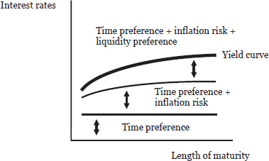
Note: Time preference is presented as being constant across the varying maturities. Some economists, like Rothbard (2009, 449), argue that time preference should be the same across time (flat), while others argue that our impatience should increase as we move further into the future (upward sloping). The reality is that time preference is so intertwined with inflation risk and liquidity preference that it can only be conceptually separated from them. No praxeological or empirical test could determine which interpretation of time preference is correct. As a result, there is no a priori answer, and the shape of the time preference curve is a result of one’s assumptions about human behavior.

Figure 18: The components of the yield curve

One significant error made by economists has been to associate a particular segment of the SOP with a particular segment of the yield curve. Suppose that an entrepreneur has a plan that will take three years to show any return. To finance this venture (financing always comes from savings—deferred consumption), the entrepreneur’s own savings, someone else’s savings, or both must be used. The options available to the entrepreneur-borrower are plentiful. The borrower could match maturities and take out one three-year loan, or the borrower could obtain three one-year loans, or two eighteen-month loans, or one two-year loan to be followed by a one-year loan, and so forth. Here is the most important part: the maturity of the loan (i.e., where it is in the TSIR) and the location of the business within the structure of production have no direct time link to each other. Figure 19 illustrates the error of assuming this direct time link. Any conclusions that stem from this faulty analysis are illegitimate.

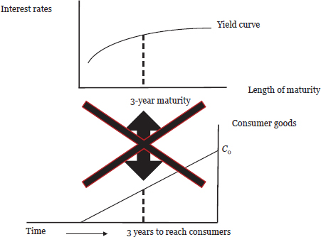
Figure 19: No direct time link between the yield curve and the SOP

UNRESOLVED PROBLEMS WITH THE ABCT

In our simple ABCT model, we assumed that monetary expansion lowers the interest rate. When we relax the assumption of a single interest rate, we can maintain the conclusion that credit expansion affects all maturities in the TSIR and in the RSIR. However, we do not know if this decrease in rates caused by monetary expansion will be evenly applied across each array of interest rates. Nevertheless, we can state that this change stimulates both consumption and investment.

Entrepreneurs use tools like net present value (NPV) in deciding whether to accept or reject an investment project. The NPV is the summation of appropriately discounted projected future returns (cash flows). The discount rate often used is the weighted average cost of capital (WACC). The WACC is a weighted average of the opportunity costs of the different types of financial capital: equity, debt, and preferred stock. A company’s opportunity cost of equity (RE) is the rate of return investors expect to receive from their equity investment in a company, a company’s opportunity cost of debt (RD) is the rate of return investors expect to receive from their purchase of a company’s bonds, and a company’s opportunity cost of preferred stock (RPS) is the rate of return investors expect to receive from their investment in a company’s preferred stock. Thus the WACC = [WE ∙ Re] + [WD ∙ RD (1 − corporate tax rate)] + [WPS ∙ RPS], where WE, WD, and Wps are the respective weights.

When there is monetary expansion, there is a change in the WACC, which promulgates a rebalancing between equity and loans. In general, the WACC falls as the opportunity cost of debt (RD) falls, and this has a greater impact on the (projected) longer-lived fixed capital goods (Cwik 2008). When longer-lived fixed capital goods are encouraged, more roundabout (complex) capital structures are undertaken throughout the SOP. More specifically, projects with longer maturities and more specific capital equipment are encouraged. The key point is that during the unsustainable boom, there is a switch from more substitutable capital to more complementary (specific) capital, making the liquidation phase deeper and more prolonged.

In our model, we saw that as the artificial boom closed and the economy neared the upper turning point, all the entrepreneurs scrambled to find bricks (real resources) to finish their projects. When the assumption of a single interest rate is relaxed, we see that there is in fact more pressure on short-term interest rates than on long-term interest rates during the upper turning point. The reason is simple: if entrepreneurs are not able to get any financing for the needed bricks, they cannot complete and sell the houses they have invested in building. If they do not sell the houses, they lose all that they have sunk into the project. Thus, they are willing to borrow at high short-term interest rates to prevent big losses. The result of this scramble for short-term funds is seen in the empirical relationship of an inverted yield curve (Cwik 2005). Historically, an inverted yield curve has preceded a recession by an average of four to six quarters.

_____________________________

Yeager (1997, 253–56) presents a sympathetic criticism of the ABCT from the perspective of a monetary disequilibrium theorist. He argues that the disturbances caused by monetary injections are insufficient to cause a business cycle.

Duration is a tool which determines the number of years (as a weighted average) that are needed to recover the purchase price of a bond based on the pattern of the cash flows over the life of the bond.

Not all companies utilize all three types of financial capital.