Austrian Business Cycle Theory

Part 2

Creating a Business Cycle Model

PRELIMINARIES

IN ORDER TO EXAMINE SOMETHING as complex as a macroeconomy, we need to simplify the important variables. A model of an economic system is an abstraction that necessarily excludes all but the most important pieces. Macroeconomists need a simple starting point. The state of equilibrium gives economists a reference point from which they can compare how some economic elements affect, and are affected by, other factors. The assumption of equilibrium means that everything in the model will continue in a balanced state (without change) until something new happens. Embedded in the notion of equilibrium is the idea that entrepreneurs do not make systemic errors. In other words, they tend to get it right. However, a business cycle is characterized by a “cluster of errors” committed by entrepreneurs (see Rothbard 2000, 8). These entrepreneurial errors are spread across the entire economy; they are not simply a gyration within a particular market sector. The source of such widespread error must be something that affects the entire economy.

There are only two elements in an economy that have such a systemic impact: money and time. Money is unique in that, with few exceptions, it touches every trade. When the supply of money increases, the value of every unit falls, though it does not do so uniformly. Because of the decrease in purchasing power, more money is needed to make the same purchases. In other words, we see an inflation of prices that affects the entire economy. Money is the prime candidate behind the mechanism that begins and propagates the business cycle.

The other element that permeates the economy is time. Most other economic schools assume that continuous production allows us to discard time as an element in macroeconomic models. A key feature of the Austrian school is its insistence that production takes time. In addition to emphasizing that there is a time structure to production, Austrians consider time as the basis of interest rates. Interest rates are intertemporal prices; that is, prices that connect the present to the future. While time does connect all economic decisions, it alone cannot be the cause of a business cycle because human beings cannot change the flow of time. Nevertheless, interest rates, which reflect our relation to time, play an important part in the swings of the business cycle.

The Basic Idea

The Austrian school states that a business cycle moves through five recognizable stages. These stages (seen in figure 2) are (1) monetary expansion, (2) unsustainable boom, (3) upper turning point, (4) liquidation phase, and (5) recovery.

In the real world, these stages are sometimes entangled and less clearly defined. In fact, due to bad economic policy, an economy might not even experience a true recovery, as was the case of the 2007–9 recession.

A Simple Story

Sometimes, the best way to convey an idea is through the use of an allegory. Imagine you are in a class and the professor says that all of the grades have been destroyed by a computer virus. This unreasonable professor says that your grade for the entire class now rests on a fifteen-page paper that is due on his desk at eight tomorrow morning! Of course, you have not started the paper. In fact, you do not even have more than a basic topic. Your other commitments prevent you from even getting to your computer until after dinner. You are tired and anxious but begin the paper. Around eleven, the adrenaline has worn off and you are feeling tired. What do you do? You brew a pot of coffee and continue. When two in the morning rolls around, you are still not done, yet the effects of the coffee have faded. You are drowsy again. You need another jolt of caffeine. Will the same amount of coffee provide the same amount of stimulation? No, it will not, and so you need to “increase the dose.” By six in the morning, you are barely able to keep your eyes open, but then you remember that you need footnotes and the bibliography! Again you have a choice, so once again, you increase your caffeine intake. Finally at eight, you slam the paper upon the professor’s desk, go home, and crash, falling soundly asleep.

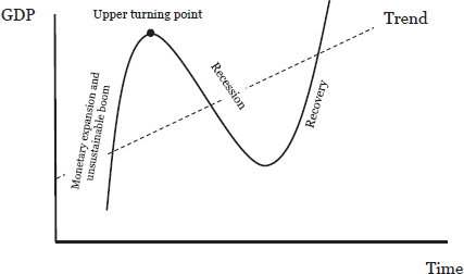
Figure 2: A business cycle

This story is an allegory for the business cycle. When credit is created and pumped into an economy, it is an artificial stimulant for the economy in the same way the caffeine is for the student. The new credit circulates through the entire body of the economy, sending false signals to all entrepreneurs. Entrepreneurs engage in ventures that are built upon the temporary stimulative credit injections. Austrians call these projects “malinvestments.” When the effects of the stimulant wear off , the monetary authorities have a choice to stop or continue. If they choose to continue, they will need to increase the dose. But eventually, there must be a crash. Either the monetary authority stops stimulating the economy, which results in a credit crunch, or the economy runs out of savings, which results in a resource crunch.

All other economic schools say that anything we can do to delay or avoid recessions is the best path. In contrast, according to Austrian business cycle theory (ABCT), the liquidation process of a recession is a necessary—although painful—step toward recovery. We have been up all night drinking too many sugary, caffeinated frappes. When the student sleeps, the time that the body uses to flush out all of the consumed stimulant and recover from the binge is essentially wasted. No other activities can be done. Similarly, the economy uses the recession to clear out the malinvested capital so that future growth will be on a firm foundation. But even if the economy returns to its precycle levels, the span of time spent in the cycle has also been wasted.

The Intermediate-Level Model

In his book Time and Money (2001), Roger W. Garrison presented an intermediate-level Austrian model of the macroeconomy. The goal of Garrison’s model is to convey the essential elements of the ABCT. The model comprises three interlocking graphs: the structure of production (SOP), the production possibilities frontier (PPF), and the loandable funds market. In the following sections, we will examine each component individually and then integrate them. Then we will apply the model to three scenarios: when people become more patient (meaning that they postpone consumption and make real resources available for investment purposes), when a price ceiling on interest rates is imposed, and when the monetary authorities expand the money supply through credit creation. This final scenario is the Austrian business cycle theory.

The Structure of Production

When something is made, it must go through a distinct process. To make a wooden table, we must first cut down the tree and then take it to a sawmill before it can be transformed into a table and sold to a customer. We cannot cut the tree into boards before we cut the tree down. There is an order to the production process. The SOP represents this order. It shows the degree of capital complementarity between the economy’s different production stages.

Of all the goods produced, only a small fraction are for consumption. However, consumption is the sole reason for production. In order to produce, certain elements must be combined. They are labor, natural resources, and time. These three components are called the “original factors of production.” Imagine a survivor alone on an island. Suppose that of all of his needs, the most pressing is hunger. The most basic element needed is the food itself. Without that, there is no chance to alleviate the survivor’s hunger. The castaway must work to acquire food. This might entail walking through the brush to get to berry plants or climbing a tree. It also must be recognized that this activity takes time.

If our survivor needs ten units of fruit a day to stay alive and can only gather five units a day, then our castaway will have a short (and probably miserable) life. If ten units can be gathered, then he will be able to live, albeit at a subsistence level. However, if more than ten units can be gathered per day, then the survivor has a choice to make. Suppose that the castaway can gather fifteen units per day. One option is to gather the ten units and then take the rest of the day off (consuming leisure).

Another option is to gather fruit for two days and take the third day off (also consuming leisure). An important alternative arises, however. What if instead of consuming leisure, he does something productive with this time? The castaway might realize that a long pole could be fashioned out of branches to knock the fruit out of the trees, making the job of gathering more productive. The creation of the pole is the creation of a capital good, which can only come about if savings are first accumulated. Capital goods are not directly serviceable, but instead are utilized in the production of finished, directly serviceable goods. There are three kinds of capital goods: capital equipment, intermediate capital (also known as goods in process) and financial capital.

Capital equipment is the category that most people think of when discussing capital. The tools, machines, and equipment that enhance our productive capabilities fall into this category. Capital goods are built by combining natural resources, labor, and time (the original factors of production), and often with other capital goods. Capital goods are embedded in specific stages of production. They work cooperatively with other factors of production. In the example of our lone survivor, the pole is capital equipment. It allows him to increase output. Suppose that output is doubled to twenty units of fruit a day. This additional output not only raises our castaway’s living standard (more fruit and/or leisure time), but also gives him more time to devote to other projects like building shelter or spear fishing.

When the survivor gathers the fruit, the berries not immediately consumed are called intermediate capital, also known as goods in process. If the berries are used as ingredients in a recipe, these berries become just one part of a greater whole. In a modern economy, most goods and services are goods in process. They are not directly consumable but are necessary components of a final, finished product.

The third type of capital is financial capital. Money is the tool by which all economic actors calculate how best to allocate goods and resources. Monetary calculations take place from the top echelons of financial markets all the way down to the most basic exchange in a farmers’ market. Monetary calculation is the tool everyone uses to decide whether to buy, sell, or wait at every level of the economy.

In figure 3, we see that there are four hypothetical stages of production. Production has a specific sequence. If we are building a wooden table, we cannot first manufacture the table and then cut down the tree. Chopping down the tree must come first. As the production process moves forward, value is added. The goods in process become more valuable as they are transformed (e.g., the tree at the sawmill is more valuable than the tree still in the forest). Ultimately, the final output emerges on the right side of the graph as a consumer good (figure 3).

All of the original factors of production (natural resources, labor, and time) are represented in the structure of production. Capital equipment is embedded in each stage of production. As goods in process flow through the SOP from left to right, this intermediate capital is combined with additional resources, labor, and preexisting capital equipment (figure 4). And while the physical goods and services are flowing from left to right, financial capital flows in the opposite direction, from right to left.

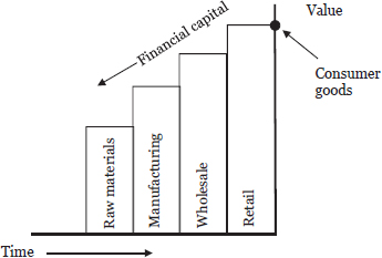
Figure 3: Structure of Production

We can think of specific forms of capital equipment as being embedded in each stage of production. In our wooden table example, we can imagine people using saws to cut the trees down and trucks to haul them out of the forest. We can imagine the giant cutting equipment at the sawmill.

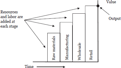
Figure 4: The role of resources and labor in the structure of production

Moreover, there are markets between the various stages of production (see figure 5). These markets are of critical importance, for they illustrate what makes complex production possible. When consumers buy from retailers, they are directly valuing consumer goods. These consumer demands communicate to the various stages of production what to produce and how much. This communication does not take place all at once. It is a step-by-step process. Because of consumer demand, retailers will demand goods from wholesalers. Wholesalers will then demand goods from manufacturers based upon the retailers’ demand, which was derived from the consumers’ demand. All the demand curves found throughout the SOP are imputed from the consumers’ original demand. Only the consumers’ demand is a direct valuation, all of the other demand curves in the SOP are ultimately derived from the consumers.

The owners of the apple orchard, the lithium mine, and other original factors of production associate an opportunity cost with the use of their resources. Opportunity costs are the sole basis of supply curves. Thus, supply curves originate with the owners of the original factors of production. These supply curves are then imputed “forward” through the SOP (along the x-axis; see figure 5).

Thus, between each and every stage, the subjective valuations of buyers and sellers interact and form prices. The intermediate capital goods flow from left to right, while financial capital flows in the opposite direction.

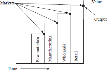
Figure 5: Structure of production with markets

Of course, there are more than four stages of production in a real economy, which is far more complex than our model. Conceptualizing the SOP as a triangle illustrates the uncountably many stages in a real economy (figure 6).

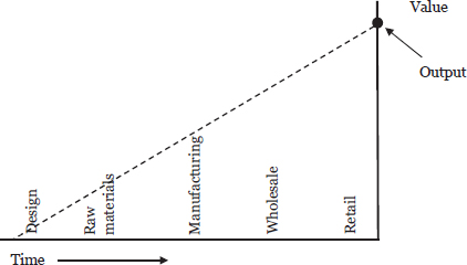
Figure 6: Structure of production as a triangle

Figure 6 lists five general stages, yet it must be emphasized that a particular company or even industry cannot be specifically located on the SOP. A complex economy uses dual-purpose goods and recursive loops. Dual-purpose goods, such as computers, can be used as both consumer goods and as capital equipment. In a recursive loop, a good creates the inputs to make a copy of itself. For example, a steel tool is used to extract iron ore, which is then used to make tools to extract more ore.While the image of a triangle by no means perfectly captures all of the aspects of a complex macroeconomy, it does capture all of the necessary elements of the SOP.

The Production Possibilities Frontier

The production possibilities frontier (PPF) assumes that, at the present state of technology and with fixed resources, there are two producible goods. Paul Samuelson (1948, 18) created one of the most famous examples of the PPF, showing the trade-off between wartime goods (guns) and civilian goods (butter). Garrison’s (2001) innovation was to replace guns and butter (both consumer goods) by making the trade-off between present goods (consumer goods) and future goods (investment goods). The PPF attempts to illustrate all of the possible combinations for maximum output in the economy.

There are two ways to display the PPF. The first illustrates the maximum potential output of an economy, while the second, Garrison’s model, shows the maximum sustainable output. While Austrians have used both versions, the Garrisonian model, though based on sustainable output, allows the economy to temporarily move beyond sustainable output, which is better for business cycle discussions (figure 7).

If the entire economy were to devote its entire production capacity to consumer goods, then it would produce at point A in figure 7. If the producers shift toward investment goods, not only will there be a reduction in the production of consumer goods, but this reduction will also follow a concave path. The reason the PPF is concave is due to the law of increasing opportunity costs. In order to move from point A to point B, the economy sacrifices five units of consumer goods. When it moves from point B to point C, a larger sacrifice (ten units) is required. As we shift along the PPF, from points A to B to C and so forth, we see that in order to gain equal increases of investment goods, we must sacrifice more consumer goods.

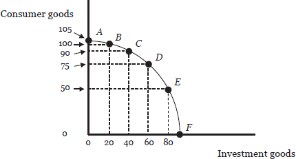
Figure 7: The Garrisonian production possibility frontier

Every point on the PPF represents a possible maximum sustainable output. Any point that is inside the PPF represents an economy below its maximum, generally meaning that it is in a recession. While we can say that being on the PPF is preferred to being in a recession, we cannot make the case that any specific point on the PPF is preferred to another point on the PPF. We can state that more consumption (less saving) today and less investment tomorrow produce less economic expansion. And we can state the inverse, that less consumption (more saving) today and more investment tomorrow produce more economic expansion. However, we cannot say that a particular point is best for an economy, despite our personal preferences.

A point beyond the PPF is possible, but it is not sustainable, in the same way that a person can stay up all night working on an economics paper (occasionally “pull an all-nighter”) but cannot stay up every night. Eventually, that person will need to sleep.

Economic growth is illustrated by an expansionary shift of the PPF. In figure 8, we begin at point A1, which represents a fully employed economy. At point A1, the economy produces C1 consumer goods and I1 investment goods. Any increase of consumer goods must come at the expense of investment goods, unless we can change the PPF boundary. The PPF expands with economic growth, such as when savings and investment fuel an increase in technology that makes more production possible. The expansion is shown by shifting the entire curve upward and to the right. While any point on this new frontier is superior to the old frontier, point A2 shows that with the use of this new technology we can potentially have both more consumer goods and more investment goods.

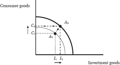
Figure 8: PPF shift showing economic growth

The Loanable Funds Market

The loanable funds market shows an economy’s aggregate rate of time preference. Time preference reflects the fact that people prefer sooner to later, ceteris paribus. If offered the choice between $100 now and the promise of a $100 a year from now, people will prefer the $100 now because it can be used now.

To model time preference, we are going to make a significant, simplifying assumption about the loanable funds market: there is only one interest rate. In our market, the interest rate is determined by time preference. Although in non-Austrian constructions of the loanable funds market the demand is also determined by subjective time preferences, the supply side is often determined by objective productivity factors. In contrast, the Austrian model of this market is premised on the theory that both the demanders and the suppliers of loanable funds are motivated only by their time preferences. This model is called the pure time preference theory (PTPT) of interest rates.

The demanders of loanable funds are those who wish to borrow. Some people have a high time preference, meaning that they are not very patient. These borrowers need the funds quickly and cannot delay their borrowing. Other borrowers have enough options, so they can wait for better rates (low time preference). A downward-sloping demand curve captures the entire array of time preferences of all those who wish to borrow loanable funds.

The suppliers of loanable funds are savers—those who are deferring consumption. The upward sloping supply curve captures their entire array of time preferences. At the lower portion of the supply curve are those who are natural savers. They need little inducement to keep them from spending. At the higher portion of the supply curve, we see people who love to spend. In order to induce them to defer their consumption, a large reward must be offered. Thus, as interest rates rise, we see an increase in the quantity of loanable funds supplied. The supply curve slopes upward.

Putting the supply and demand curves together, we create a model of the loanable funds market (figure 9). The vertical axis measures the intertemporal price that emerges—the interest rate. Along the horizontal axis, we see the quantity of loanable funds supplied and demanded in the market. In equilibrium, there is an interest rate (i1) that balances the quantity supplied (savings, S1) with the quantity demanded (investment, I1).

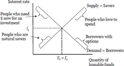
Figure 9: The loanable funds market

The result is a market that reflects the time preference of its society. As indicated above, other schools of economics include the objective factor of productivity, but the Austrians do not.

The question “Why not include productivity?” needs to be examined. First, a distinction between rents and interest returns must be made. Every factor of production earns a return—a rent. This rent is the price that must be paid to the owner of a factor of production. In equilibrium, every factor earns a return (rent) that is equal to its marginal product. The marginal productivity of a piece of capital equipment explains the height of its rental price. However, the marginal productivity does not explain why these rents should be discounted across time. A change in the productivity of a capital good will change its rent, but not the rent’s discount rate across time (the rate of interest). The discount rate is separate and independent from the productivity of the capital good. Thus, interest rates are based upon time preference, and rents are based upon a factor’s productivity.

Putting the Models Together

The Garrisonian model of a macroeconomy interlocks the three preceding graphs (figure 10).

We begin in the lower right, with the loanable funds market. In this market, savers and borrowers come together. At interest rate i0, the quantity of loanable funds supplied (S0) matches the quantity of loanable funds borrowed and invested (I0). It is important to emphasize that the amount of investment depends upon the amount of savings; saving is the first step in the “magic” formula for economic growth.

The amount of funds used to create investment goods (I0) is connected to the PPF by the corresponding horizontal axes. In equilibrium, the economy is at full employment, so we find the economy at point A0 on the frontier. At point A0, the corresponding amount of consumption goods produced is C0. Finally, C0 links with the SOP (in the upper left ). The slope of the SOP reflects the rate of time preference (the interest rate) in the economy. It is from this equilibrium that we start our macroeconomic analysis.

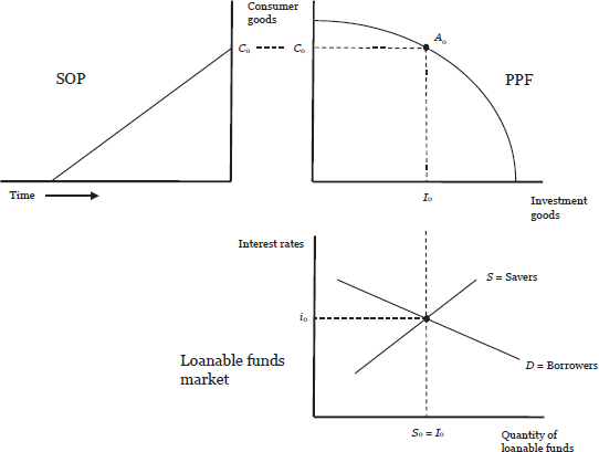
Figure 10: The Garrisonian macroeconomic model

SCENARIO 1 PEOPLE BECOME MORE PATIENT

Now let us put this model into action and demonstrate how it works. Suppose that people become more patient. In other words, they become more willing to save and to defer consumption. The first implication of this change will be found in the loanable funds market. The supply of loanable funds will shift to the right, lowering the equilibrium interest rate and increasing the quantity of loanable funds saved and borrowed (figure 11).

With more borrowed funds allocated toward the construction and implementation of investment goods, we move along the PPF. There is an increase in investment goods and a decrease in consumer goods.

Note that this conclusion completely differs from mainstream economic analysis. Mainstream economic analysis looks at gross domestic product (GDP), which is calculated by adding the following components: consumption spending, investment spending, government spending, and net export spending. Consumption spending makes up about two-thirds of the total GDP. In the mainstream models, the increase in investment spending does not make up for the decrease in consumption spending, so the GDP statistic falls with less consumer spending. Since the GDP statistic is the prime measure of the well-being of the economy not only for economists but also for politicians and journalists, there is a strong political incentive to prevent GDP from falling.

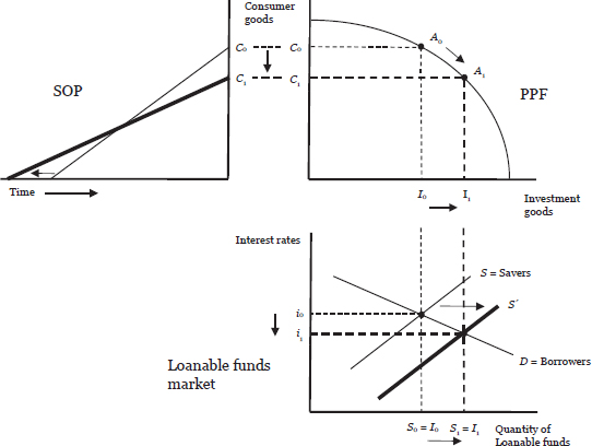
Figure 11: People become more patient

As we move along the PPF, we see that even though the whole economy remains at full employment, there are changes in many sectors. These changes are visible in the SOP (figure 12).

With a reduction in demand for consumer goods (because people are becoming more patient) comes a decrease in demand for late-stage goods (all those goods that are closer to the consumers). While demand for consumer and late-stage goods is falling, savings are being borrowed and employed in more complex production patterns. While an expansion of investment goods can take place at any and all points in the current SOP, the addition of production complexity is illustrated by a lengthening of the structure of production. We can see the micro-economic effects of these changes in figure 12.

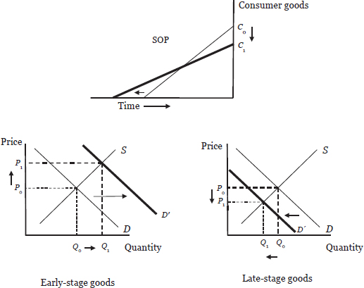
Figure 12: Changes in the structure of production

What does lengthening the SOP mean, and why does the SOP lengthen when there is an increase in savings? To describe how economic growth comes from the addition of capital goods, Austrians have used several terms, including higher degrees of roundaboutness, increasing complexity, capital deepening, and lengthening the SOP. The idea begins with the observation that adding complexity to a production process for its own sake is wasteful. The only reason to make a production process more complex is because it yields a benefit; namely, higher profits. Increasing complexity can manifest as a faster assembly line, higher-quality products, more diverse products, and so forth. When a car was designed in the past, draftsmen were employed to draw the plans for each part of it by hand. Any changes to the plans would require many labor hours of redrawing. Today, these changes are made very quickly using computer programs. So while we have the ability to make changes to designs much faster, the process is actually more complex. Someone had to engineer the design program. Someone had to build the computers. Someone had to design the computers. Many stages of production necessarily precede the modern draftsman’s work. These extra stages make the production process more complex—longer—but they also make it more efficient.

Decreases in consumption free up resources to shift from one sector of the economy to another. This freeing up of resources grants entrepreneurs the time and wherewithal to engage in new productive projects. These projects—new stages of production—add complexity to the economy. To illustrate these additional stages of production, we graphically extend the economy’s entire SOP as seen in figure 12. However, this extension does not mean that any specific economic sectors (like forestry) will always expand as people become more patient.

The model that we are using is called a comparative static model, meaning that it only captures points in time. However, the process that we are attempting to describe takes place through time. One of the key results that was left out of figure 12 is that savings and investment lead to economic growth. To illustrate economic growth, we need to add another step to the comparative static model. As investors use saved funds to lengthen the SOP, the gains in productivity will push the PPF outward (as seen in figure 13). As described above, these economic improvements benefit the entire society. The SOP will shift outward along with economic growth but not smoothly. It will move in a piecemeal fashion. Some sectors will expand while others lag. Furthermore, as new business ventures begin, there will also be an increase in the demand for loanable funds. Initially, the interest rate will fall as people become more patient. However, as more investment projects become feasible, there will be an increase in the demand for loanable funds, shifting the demand curve from D to D’. In figure 13, we are supposing that the interest rate returns to i0, but this is just to keep the graph clean. There is no a priori method to determine where the final-equilibrium interest rate will be. However, we can say that higher savings rates will push the PPF out at a faster rate than lower savings rates.

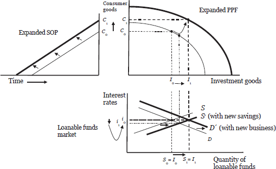
Figure 13: The macroeconomy with economic growth

One final point: We are using a comparative statics model, which captures only moments in time, to show economic growth; however, there is no resting equilibrium for economic growth. What we are attempting to describe using static models is a dynamic process.

SCENARIO 2 IMPOSING A PRICE CEILING ON INTEREST RATES

Suppose that the government has decided to place a ceiling on interest rates. As seen in figure 14, if the ceiling is placed below the market interest rate, a shortage of loanable funds will emerge. The lower interest rate sets in motion two reactions. Savers reduce their savings (from S0 to S2; we move along the supply curve) and increase their consumption (from C0 to C2). Entrepreneurs, on the other hand, see a lower cost to borrowing and thereby attempt to increase their borrowing (from I0 to ID; we move along the demand curve). This attempt to borrow more creates a gap between the quantity of loanable funds that borrowers would like and the amount actually saved and available. The result is a credit shortage.

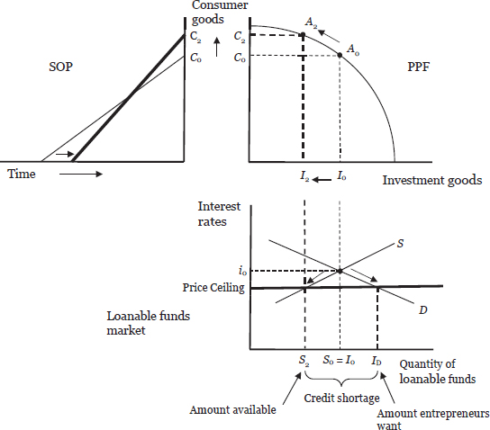
The credit shortage does not allow the investors to borrow as much as they would like. In fact, with a lower savings rate, the amount actually borrowed and invested decreases (from I0 to I2). We see the impact of the change in the PPF. The equilibrium point moves counterclockwise along the frontier (from A0 to A2). Although the economy is still at full employment, the underlying conditions have changed. People are consuming at a higher rate (C0 has shifted to C2) and the SOP has become less complex. In effect, what we get is a bust without a boom.

SCENARIO 3 THE BUSINESS CYCLE

Stage 1: Monetary Expansion

Austrian business cycle theory (ABCT) begins with assuming the economy to be in a harmonious equilibrium state. In other words, there is a balance that will continue until something changes. This change can be endogenous (like a simple change in tastes and preferences) or exogenous (like a new government policy). As pointed out above, Austrian economists postulate that money is the only ubiquitous economic element that can cause a cycle.

The business cycle begins with an expansion of the money supply. There have been times in history when the money supply has expanded either through conquest or through the discovery of new deposits of precious metals. The business cycles caused by these expansions depended upon the size and duration of the influx of new money. Today, no country uses precious metals as its money, and these older roots of monetary expansion are no longer a concern. Today’s money is called “fiat money.” It is money that is backed by nothing other than the promise of a government.

The ABCT posits that a monetary authority, usually a central bank, engages in a policy of monetary expansion. While the reasons for this policy range from misguided economic theory to political gains, the reason why the central bank adopts an expansionist monetary policy is not relevant to our model. It is the fact that the central bank expands the money supply that matters.

Under modern monetary systems, the typical method to expand the money supply is to create and inject credit into the banking system. While the particulars may differ with location and time, the effects tend to be the same: credit expansion has a great impact on the interest rate markets. The creation and injection of credit causes the supply of loanable funds to shift to the right (S to S’ as seen in figure 15). The effect of adding new money to the market is a reduction of the interest rate. The lowering of the interest rate is a movement along the demand curve: at this new and lower rate, more investors want to borrow money and finance new projects (I0 shift s to I1). Yet what cannot be overlooked is that the addition of new money does not lower the time preferences of savers. On the contrary, as those who are saving (deferring consumption) watch interest rates fall, they will save less (S0 shift s to S1). As savings fall, consumption will increase. Normally, when both the interest rate and the quantity of loanable funds available fall, we see a credit shortage develop (as we did in scenario 2). However, in our scenario, this credit shortage is covered by the creation of new credit. This credit comes from nothing. It is literally typed into existence on computers. As a result, we see a separation emerge between actual savings and the amount invested.

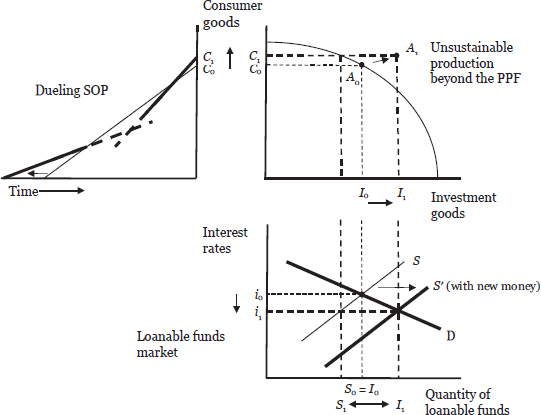
Figure 15: The unsustainable boom

Stage 2: Unsustainable Boom

The interest rate is an intertemporal price that connects today with tomorrow. In January 2001, the effective federal funds rate—the major interest rate that the U.S. central bank targets—was at 5.98 percent. Suppose that an entrepreneur, Sam, was considering a business plan projected to yield a 4.00 percent return. At that interest rate, Sam would have shelved the project and simply put the money in a savings account to gain the higher rate of return. Now suppose that the central bank was to engage in an expansionist monetary policy, which reduces the interest rate. In December 2003, for instance, the effective federal funds rate fell to 0.98 percent. Now what would Sam decide if given the same choice? In this case, it is not only rational for Sam to begin the project, but it is his fiduciary duty to pursue the highest rate of return for his business.

The effects of this rate change are far reaching. The interest rate is sending a false signal to entrepreneurs across the whole economy. It is telling entrepreneurs throughout the entire SOP to begin new capital projects which otherwise would not have appeared worth pursuing.

These projects that entrepreneurs are misled into starting are called malinvestments. There is no a priori method to determine which particular projects are malinvestments and which are not. This is because money is fungible, so there is no method to determine which money is the newly created credit and which existed before.

At the same time as a malinvestment boom begins (as investment in figure 15 shift s from I0 to I1), there is a boom in consumption (an increase from C0 to C1). As a result of the increase in both consumption and investment, a shift to a point outside of the PPF (from point A0 to A1) occurs, representing an unsustainable boom. This boom is similar to how a person is able to stay up all night but not every night.

We can conclude that the point outside of the PPF is unsustainable by examining the effects of the monetary expansion on the SOP. A decrease in interest rates resulting from credit expansion causes the general public to change its savings-consumption ratio. A lowering of the interest rate encourages people to consume more and save less. The SOP reflects people’s increasing consumption by shifting upward, which steepens its right segment, the segment closest to the consumers (the shift creates the partially dashed line starting at point C1 in figure 15). This steepening of the right segment of the SOP shows the change in the savings-consumption ratio. The dashed portion of the shifted right segment indicates the direction people’s new preferences would lead if they were able to be fully implemented. In other words, consumers are less patient and want more consumer goods now. Only a shorter, less complex, SOP can accommodate these desires.

At the same time that people are consuming more, investors are building more complex capital structures in the economy. They are receiving (false) signals that indicate the general public has more patience to wait for more consumer goods to be produced in the long term (as seen in scenario 1). The entrepreneurs incorrectly believe that they can build a more complex economy and lengthen the SOP. The SOP segment on the left shows the entrepreneurial expansion of building projects. This segment has flattened to indicate the entrepreneurs’ (false) perception of the capital structure. The dashed portion of the shifted left segment shows the direction of the SOP if it were to be fully built out under these conditions.

When the two segments of the SOP fail to align, a “dueling structure of production” results. The SOP is in disequilibrium and, consequently, is not in a state of rest, meaning that something must change. The boom is unsustainable.

Stage 3: Upper Turning Point

A famous business cycle example—used by Mises—begins with a master builder whose task is to erect buildings using a finite amount of building materials. Suppose that this builder is using bricks to build houses. If the builder has enough bricks to complete four houses, can he begin to build six houses? Yes, but there are not enough bricks to complete all the houses (see figure 16).

In Mises’s example, the lower interest rate tempts the builder to start more buildings than he is currently capable of finishing. The interest rate misguides the builder into believing that consumers are more patient—reducing their demand for consumer goods, which frees up resources for investment goods—than they are. To complete all of the homes after he has started them, the builder will have to get more bricks. Unfortunately, this particular builder is not alone. The situation is the same for all producers. While the shortage of credit was covered through a false expansion of the money supply, the shortage of real resources is genuine. The supply of savings (represented by the bricks that it has been used to purchase) has not increased (as was miscommunicated to the builder) but has actually fallen. Upward pressure is placed upon the price of bricks, one of the input goods for the buildings. As prices rise, entrepreneurs with partially completed projects look for additional financing to meet these higher costs. Interest rates rise.

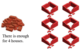
Figure 16: Malinvesting capital inputs

The economy experiences upward movements of both the interest rate and input prices.

We are at the upper turning point. The entrepreneurial “cluster of errors” has been exposed. Entrepreneurs were misled by an artificially low interest rate. The interest rate was artificially low because of expansionary monetary policy, a decision made by nonmarket participants (central bankers and politicians). The entrepreneurs miscalculated because of the actions of central bankers and politicians.

At the upper turning point, the monetary authorities are in a dilemma and have a choice to make. They can address either the issue of the increasing interest rate or the issue of increasing prices, not both. To stem the increase in interest rates, the monetary authorities can accelerate the rate of monetary expansion—as the student increases the amount of caffeine to finish the paper—or the central bank can address the increasing prices by slowing or halting monetary expansion. A reduction in monetary expansion will result in even higher rates of interest, exacerbating the builder’s situation. Politically, accelerating the monetary expansion is the preferred alternative. The reckoning can be delayed, and the consequences of the expansionary policy can be postponed. Regardless of the choice taken by the monetary authorities, the economy is in a disequilibrium, a boom which cannot last forever. Whichever choice the central bank makes, it will not achieve a “soft landing.” Recession is inevitable.

Stage 4: Liquidation (Recession)

If the monetary authorities continue to accelerate the rate of monetary expansion, the economy will eventually run out of bricks (savings). The result will be a real resource crunch. If the monetary authorities decide to stop increasing the interest rate, the result will be a credit crunch. Each of these paths leads to an economic crisis. Either the builder sees input prices rising and can no longer afford to complete the project, which results in the project’s termination and the components’ liquidation or the builder sees the interest rate become so high that the project is no longer viable, which results in its termination and the materials’ liquidation. In August 2006, the federal funds rate climbed to 5.25 percent. The result was the 2007–9 recession. If Sam, the entrepreneur we met in stage 2, had seen this high rate, he would have realized that his project, which only yields a 4 percent rate of return, was no longer viable and must be discontinued.

During the liquidation stage, those firms that invested during the malinvestment boom begin to suffer economic losses. In figure 17, we see the path of a recession. As businesses pull out of the loanable funds market, either by choice or due to an inability to continue operating (from losses), we see a left ward shift in the demand for loanable funds (D to D”). At the same time, we see that savers are also pulling out of the market (S’ to S”). Many former savers are now unemployed, as projects have been canceled, while other former savers are businesses who no longer have the funds to reinvest into the company. Note that the interest rate (i2) is shown to be equal to the initial rate (i0), but this is merely to keep the graph from becoming too cluttered. There is no a priori reason why the interest rate should return to the same level it was before the monetary expansion. The important characteristic of the loanable funds market in this stage is the level of savings. Savings are the floor upon which the level of investments falls (I1 to I2).

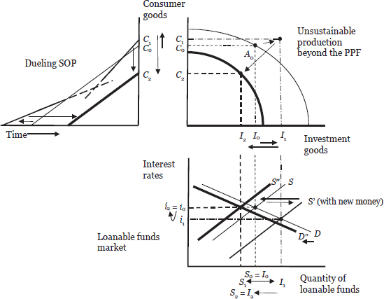
Figure 17: The recession

We can track the decrease in investment goods in the PPF (also shifting from I1 to I2). As people lose their jobs, we see a fall in consumption goods (from C1 to C2). As many capital projects are halted, many capital goods that cannot be repurposed are thrown away. Their productive capacity is lost. The entire sustainable productive capacity of the economy shrinks and the PPF contracts to a lower level. Finally, we see the contraction of the SOP. In figure 17, the new SOP is parallel to the original, but note that this is only because of the assumption that the new interest rate (i2) matches the original (i0). There is no a priori reason for the two SOPs to be parallel.

The liquidation phase is a painful, yet necessary, consequence of the preceding expansionist monetary policy. The economy has been pushed into an unsustainable boom and requires correcting. A recession is the process by which an economy converts malinvestments into productive capital, which becomes the foundation for future economic growth. Only the Austrian school argues that liquidation is a necessary condition for recovery.

In order for the economy to recover, the liquidation of failed companies must be completed. As companies fail, their assets are sold and the proceeds are distributed to the creditors and the owners. When these assets are sold, they are sold to other firms at a discounted rate. Because these firms have purchased the capital equipment at a discount, they now have the ability to turn an economic profit, even at the previous prices. For example, suppose that in the 2007–9 recession, the U.S. government truly allowed General Motors to go bankrupt. If GM had been forced to liquidate its assets, it would have had to sell its brands and divisions. There was still value in Corvette and Cadillac. Who would have bought these brands? Perhaps Toyota, BMW, or Elon Musk. It does not matter. A bidding process would have taken place, and one of the bidders would have bought Cadillac. However, the buyer does not have to pay full price in a liquidation sale. The buyer could have gotten Cadillac for pennies on the dollar. The implication is that Cadillac’s new owner could turn on the same machines and produce the same cars as GM did. However, since the new owner has a lower cost structure (having bought the division at a discount), the new owner can make a profit where the old owners could not.

This liquidation process is how malinvestments are converted into new fixed capital equipment. Unfortunately, not all malinvestments can be converted back into productive assets. Those assets that cannot be converted are thrown away. Their productive capacity has been wasted and can never be recovered. Additionally, even if the economy ends up at the same starting point, time has been lost, which is also unrecoverable. Finally, many people have lost jobs and suffered through financial, housing, and food insecurity. These hardships are real and have a human cost that is simply not calculable. They are the main reason why business cycles should be avoided.

Stage 5: Recovery

The liquidation process is necessary for normal economic growth to resume. There is no categorical difference between a recovery and normal economic growth. Both must follow the “magic” formula for economic growth.

Some have argued that Austrian economists have no policy prescriptions to offer. This notion is untrue. The most important policy recommendation is to not start down the path of monetary expansion. Expansionist monetary policy starts the artificial boom and the consequent collapse. If the monetary expansion can be avoided, then business cycles can be prevented.

What can be done once we have begun a business cycle? An important point to recognize is that the boom and the bust do not have to be symmetrical, meaning that the size of the bust does not have to equal the size of the boom. Governments can make the bust much worse than it has to be (as seen in the 1929–39 depression). Governments can make the recession longer than it has to be (as seen in the anemic recovery in the U.S. after 2009 and in Japan during the 1990s). Alternatively, governments can accelerate the recovery (as seen in the 1920–21 recession, discussed below).

Governments often make bad policy choices when dealing with a recession. Typically, to prevent an economic downturn, the monetary authority will accelerate the rate of monetary expansion. This step does not cure a recession; instead, it delays the consequences of the artificial boom, swells the number of malinvestments in the economy, and usually makes the eventual recession worse. Furthermore, governments also tend to prop up failing businesses, thereby preventing the liquidation process. The spending used to prop up failing businesses shift s resources away from more productive firms and into less productive ones. By preventing the liquidation process, the government locks the economy into an unproductive capital structure. Governments should recognize that the malinvestments need to be liquidated as quickly as possible. Instead of locking the economy into an unproductive capital structure, governments should make it easier for businesses to conduct mergers and acquisitions. By making the capital structure more malleable, governments allow resources to be shifted into more productive arrangements—creating a strong foundation for economic growth.

Governments also pay people to not work, in the form of unemployment compensation. While these policies might seem humane, they extend unemployment. People delay taking an available job, hoping to find the “perfect” job. Monetary expansion, propping up failing businesses, and unemployment compensation were all enacted in the Great Depression, in the recession of 2007–9, and throughout the 1990s in Japan. In contrast, when a recession came about in January 1920, Congress actually shrunk the size of the federal budget. The result was that resources that were previously consumed by the federal government were released for use in the private sector.

The key to economic recovery (and growth) is the amount of savings. The more savings, the faster the recovery. Policies that discourage savings prolong and deepen the recession. There are two very basic policies that can increase the amount of resources available for the private sector: cutting the size and scope of the federal budget and cutting the amount of tax revenue collected. As we have seen, when the government took a step back in the 1920–21 recession, resources were freed up to be used by the private sector. It was like adding savings directly into the economy.

When governments believe they must show that they are “doing something,” a debate arises over the array of policies that should be adopted. Any policy that favors saving over consumption (like cutting taxes on savings, investments, and corporate retained earnings) will shift resources into expediting the recovery. Policies that favor spending at the expense of saving (like stimulus checks) will shift resources away from expediting the recovery—prolonging and possibly deepening the recession.

Furthermore, for businesses, tax cuts are better than stimulus. Suppose that a firm is experiencing a $2,000 shortfall every month. Assuming constant costs and a gross margin (net sales minus cost of goods sold) of 25 percent, the amount in additional sales needed to cover that shortfall is $8,000 per month. Turning the business’s malinvestment into a sustainable capital structure will take either $8,000 of direct and sustained monthly government purchases or a reduction in taxes of only $2,000 per month. Thus, in general, the tax-cut approach will place a lower burden on the government (the taxpayer) and still yield the same result.

SUMMATION

The ABCT is a model that shows the cause of the business cycle, the reasons why it affects the entire economy, the instability of the artificial boom, the cluster of errors found at the upper turning point of the cycle, and the necessity of the liquidation phase, and that points to time-tested methods for recovery. It is a comprehensive theory that has a beginning, a middle, and an end, and it is also backed by empirical studies. The attempts to refute of the ABCT tend to either criticize the empirical studies or create caricatures of the ABCT. We will explore these criticisms in part 3.

On the other hand, modern macroeconomic theory presents itself in the form of a bicyclist who has been hit by a car. The modern theory is really two separate and independent models. The first model is a theory of a boom and a return, while the second is a theory of a collapse and a return. Modern macroeconomic theory does not really have a business cycle theory. In contrast, the Austrians have a theory that presents a coherent story (which is supported by historical cases), has a defined cause and cure, and can answer several more questions.

The ABCT is not perfect. The model presented above is a simplified version of the theory. When some of these assumptions are relaxed, complications arise. These difficulties are not so much problems with the theory as they are complexities that require further thought and clarification. It is to these unresolved problems that we now turn.

_____________________________

Money is not neutral, meaning that changes in purchasing power are not instantaneous nor even. Changes in value take place at particular points first. The wave of changes is like honey spreading slowly across a surface as it is poured out. Hayek (2012, 326) used this analogy in a technical debate. For a very readable article on the nonneutrality of money, see Mises (1990b).

This retelling follows my article “The Economy Pulls an All-Nighter,” which appeared in the Mises Daily on September 29, 2003.

The latter two components are usually found in principles-level textbooks, which makes the concepts more accessible to beginning students.

Capital complementarity is the degree to which specific capital goods work together. Opposite to capital complementarity is substitutability, which is the degree to which goods can be used in lieu of another. For further discussion, please see part 3.

Recursive loops and other complicating factors will be examined in part 3.

Samuelson (1948, 18) states, “Let us, therefore, simplify (idealize, abstract) and assume that there are only two different goods or classes of goods to be produced. For dramatic purposes, let us consider the famous pair, butter and guns, two commodities popularly used to illustrate the wartime problem of choosing between civilian and military production.” However, Samuelson did not create the PPF. For example, Gottfried Haberler ([1933] 1959, 176) used a PPF in his discussion about international trade fifteen years earlier.

Some people might argue against the idea that time preference always has a positive rate by stating that they prefer lunch at lunchtime and not now. This example violates the ceteris paribus restriction. The ceteris paribus caveat means that we are assuming that all other factors are held constant. When a person says that they would rather wait until lunchtime to have lunch, they are not holding all other factors constant. A rather important factor, one’s hunger, changes between now and lunchtime.

Unfortunately, it is a static model, meaning that it captures a snapshot in time. As we use the model, we need to keep in mind the dynamic nature of these elements.

Rothbard (2009, 517–27) demonstrates how the increase of net investment necessarily lengthens the SOP.

Some have argued that widely used goods such as oil or energy can cause a business cycle. Despite how widely used such goods are, they cannot be the cause of a systemic cycle. A reduction in the supply of widely used resources will certainly cause disruptions and shift resources, but a cycle exhibits a systemwide up and down.

John P. Cochran (2001, 19) was the first to use the phrase “dueling production structures.”

See Mises (1998, 557).

Please see the section “Unresolved Problems in the ABCT” below for an explanation of how this process necessarily leads to an inverted yield curve.

The change in the cost of inputs is more impactful than the increase in interest rates. The increase in the cost of inputs has a one-to-one impact, meaning a 25 percent increase in input prices leads to a 25 percent increase in the amount of financing required. For example, if my cost of bricks increases from $100 to $125, I need an extra $25 to finish my production project. However, a 25 percent increase in interest rates (from 4 percent to 5 percent) has an impact of much less than 25 percent. As the crunch intensifies, 15–20 percent of the collapse in profit margins around the economy is due to the increase in interest rates, but approximately 80 percent is due to the rise in input prices. See Cwik (2008).

While it is important to note that the monetary inflation should stop, deflating the money supply to its previous level is also not a solution. Mises (1990, 76) said such a policy would be like after running a person over and then, to fix it, backing the car over him again.

The Democrats had lost control of the House and Senate in the 1918 midterm elections. Furthermore, President Woodrow Wilson had suffered a stroke in September 1919. When the 1920 recession hit in January, Wilson was unable to oppose the budget-balancing cuts in federal expenditures imposed by the new Republican majorities. Federal revenue (R) and expenditures (E) for the years 1918–22 were as follows: $3.6 million (R), $12.7 million (E) in 1918; $5.1 million (R), $18.5 million (E) in 1919; $6.6 million (R), $6.4 million (E) in 1920; $5.6 million (R), $5.1 million (E) in 1921; $4.0 million (R), $3.2 million (E) in 1922 (“US Federal Budgetary Spending by Year,” Polidiotic, last updated March 14, 2023, http://www.polidiotic.com/by-the-numbers/us-federal-deficit-by-year/). Congress also engaged in a series of tax rate cuts, reducing the top marginal rate from 73 percent in 1920 to 58 percent in 1921, 46 percent in 1923, and 25 percent in 1924. Notice that the Congress did not cut tax rates until after it first shrank expenditures and balanced the budget.

Two full-length studies that apply the ABCT to the 2007–9 business cycle are Thomas Woods’s Meltdown (2009) and Harry Veryser’s It Didn’t Have to Be This Way (2012).