Man, Economy, and State with Power and Market

UP TO THIS POINT, WE have been investigating the rate of interest as it would be determined in the evenly rotating economy, i.e., as it always tends to be determined in the real world. Now we shall investigate the pricing of the various factors of production in the same terms, i.e., as they tend to be in the real world, and as they would be in the evenly rotating economy.

Whenever we have touched on the pricing of productive factors we have signified the prices of their unit services, i.e., their rents. In order to set aside consideration of the pricing of the factors as “wholes,” as embodiments of a series of future unit services, we have been assuming that no businessmen purchase factors (whether land, labor, or capital goods) outright, but only unit services of these factors. This assumption will be continued for the time being. Later on, we shall drop this restrictive assumption and consider the pricing of “whole factors.”

In chapter 5 we saw that when all factors are specific there is no principle of pricing that we can offer. Practically, the only thing that economic analysis can say about the pricing of the productive factors in such a case is that voluntary bargaining among the factor-owners will settle the issue. As long as the factors are all purely specific, economic analysis can say little more about the determinants of their pricing. What conditions must apply, then, to enable us to be more definite about the pricing of factors?

The currently fashionable account of this subject hinges on the fixity or variability in the proportions of the combined factors used per unit of product. If the factors can be combined only in certain fixed proportions to produce a given quantity of product, it is alleged, then there can be no determinate price; if the proportions of the factors can be varied to produce a given result, then the pricing of each factor can be isolated and determined. Let us examine this contention. Suppose that a product worth 20 gold ounces is produced by three factors, each one purely specific to this production. Suppose that the proportions are variable, so that a product worth 20 gold ounces can be produced either by four units of factor A, five units of factor B, and three units of factor C, or by six units of A, four units of B, and two units of C. How will this help the economist to say anything more about the pricing of these factors than that it will be determined by bargaining? The prices will still be determined by bargaining, and it is obvious that the variability in the proportions of the factors does not aid us in any determination of the specific value or share of each particular product. Since each factor is purely specific, there is no way we can analytically ascertain how a price for a factor is obtained.

The fallacious emphasis on variability of proportion as the basis for factor pricing in the current literature is a result of the prevailing method of analysis. A typical single firm is considered, with its selling prices and prices of factors given. Then, the proportions of the factors are assumed to be variable. It can be shown, accordingly, that if the price of factor A increases compared to B, the firm will use less of A and more of B in producing its product. From this, demand curves for each factor are deduced, and the pricing of each factor established.

The fallacies of this approach are numerous. The chief error is that of basing a causal explanation of factor pricing on the assumption of given factor prices. On the contrary, we cannot explain factor prices while assuming them as given from the very beginning of the analysis.1 It is then assumed that the price of a factor changes. But how can such a change take place? In the market there are no uncaused changes.

It is true that this is the way the market looks to a typical firm. But concentration on a single firm and the reaction of its owner is not the appropriate route to the theory of production; on the contrary, it is likely to be misleading, as in this case. In the current literature, this preoccupation with the single firm rather than with the interrelatedness of firms in the economy has led to the erection of a vastly complicated and largely valueless edifice of production theory.

The entire discussion of variable and fixed proportions is really technological rather than economic, and this fact should have alerted those writers who rely on variability as the key to their explanation of pricing.2 The one technological conclusion that we know purely from praxeology is the law of returns, derived at the beginning of chapter 1. According to the law of returns, there is an optimum of proportions of factors, given other factors, in the production of any given product. This optimum may be the only proportion at which the good can be produced, or it may be one of many proportions. The former is the case of fixed proportions, the latter of variable proportions. Both cases are subsumed under the more general law of returns, and we shall see that our analysis of factor pricing is based only on this praxeological law and not on more restrictive technological assumptions.

The key question, in fact, is not variability, but specificity of factors.3 For determinate factor pricing to take place, there must be nonspecific factors, factors that are useful in several production processes. It is the prices of these nonspecific factors that are determinate. If, in any particular case, only one factor is specific, then its price is also determined: it is the residual difference between the sum of the prices of the nonspecific factors and the price of the common product. When there is more than one specific factor in each process, however, only the cumulative residual price is determined, and the price of each specific factor singly can be determined solely by bargaining.

To arrive at the principles of pricing, let us first leap to the conclusion and then trace the process of arriving at this conclusion. Every capitalist will attempt to employ a factor (or rather, the service of a factor) at the price that will be at least less than its discounted marginal value product. The marginal value product is the monetary revenue that may be attributed, or “imputed,” to one service unit of the factor. It is the “marginal” value product, because the supply of the factor is in discrete units. This MVP (marginal value product) is discounted by the social rate of time preference, i.e., by the going rate of interest. Suppose, for example, that a unit of a factor (say a day’s worth of a certain acre of land or a day’s worth of the effort of a certain laborer) will, imputably, produce for the firm a product one year from now that will be sold for 20 gold ounces. The MVP of this factor is 20 ounces. But this is a future good. The present value of the future good, and it is this present value that is now being purchased, will be equal to the MVP discounted by the going rate of interest. If the rate of interest is 5 percent, then the discounted MVP will be equal to 19 ounces. To the employer—the capitalist—then, the maximum amount that the factor unit is now worth is 19 ounces. The capitalist will be willing to buy this factor at any price up to 19 ounces.

Now suppose that the capitalist owner or owners of one firm pay for this factor 15 ounces per unit. As we shall see in greater detail later on, this means that the capitalist earns a pure profit of four ounces per unit, since he reaps 19 ounces from the final sale. (He obtains 20 ounces on final sale, but one ounce is the result of his time preference and waiting and is not pure profit; 19 ounces is the present value of his final sale.) But, seeing this happen, other entrepreneurs will leap into the breach to reap these profits. These capitalists will have to bid the factor away from the first capitalist and thus pay more than 15 ounces, say 17 ounces. This process continues until the factor earns its full DMVP (discounted marginal value product), and no pure profits remain. The result is that in the ERE every isolable factor will earn its DMVP, and this will be its price. As a result, each factor will earn its DMVP, and the capitalist will earn the going rate of interest for purchasing future goods with his savings. In the ERE, as we have seen, all capitalists will earn the same going rate of interest, and no pure profit will then be reaped. The sale price of a good will be necessarily equal to the sum of the DMVPs of its factors plus the rate of interest return on the investment.

It is clear that if the marginal value of a specific unit of factor service can be isolated and determined, then the forces of competition on the market will result in making its price equal to its DMVP in the ERE. Any price higher than the discounted marginal value product of a factor service will not long be paid by a capitalist; any price lower will be raised by the competitive actions of entrepreneurs bidding away these factors through offers of higher prices. These actions will lead, in the former case to the disappearance of losses, in the latter, to the disappearance of pure profit, at which time the ERE is reached.

When a factor is isolable, i.e., if its service can be separated out in appraised value from other factors, then its price will always tend to be set equal to its DMVP. The factor is clearly not isolable, if, as mentioned in note 3 above, it must always be combined with some other particular factor in fixed proportions. If this happens, then a price can be given only to the cumulative product of the factors, and the individual price can be determined only through bargaining. Also, as we have stated, if the factors are all purely specific to the product, then, regardless of any variability in the proportions of their combination, the factors will not be isolable.

It is, then, the nonspecific factors that are directly isolable; a specific factor is isolable if it is the only specific factor in the combination, in which case its price is the difference between the price of the product and the sum of the prices of the nonspecific factors. But by what process does the market isolate and determine the share (the MVP of a certain unit of a factor) of income yielded from production?

Let us refer back to the basic law of utility. What will be the marginal value of a unit of any good? It will be equal to the individual’s valuation of the end that must remain unattained should this unit be removed. If a man possesses 20 units of a good, and the uses served by the good are ranked one to 20 on his value scale (one being the ordinal highest), then his loss of a unit—regardless of which end the unit is supplying at present—will mean a loss of the use ranked 20th in his scale. Therefore, the marginal utility of a unit of the good is ranked at 20 on the person’s value scale. Any further unit to be acquired will satisfy the next highest of the ends not yet being served, i.e., at 21—a rank which will necessarily be lower than the ends already being served. The greater the supply of a good, then, the lower the value of its marginal utility.

A similar analysis is applicable to a producers’ good as well. A unit of a producers’ good will be valued in terms of the revenue that will be lost should one unit of the good be lost. This can be determined by an entrepreneur’s knowledge of his “production function,” i.e., the various ways in which factors can technologically be combined to yield certain products, and his estimate of the demand curve of the buyers of his product, i.e., the prices that they would be willing to pay for his product. Suppose, now, that a firm is combining factors in the following way:

4X + 10Y + 2Z → 100 gold oz.

Four units of X plus 10 units of Y plus two units of Z produce a product that can be sold for 100 gold ounces. Now suppose that the entrepreneur estimates that the following would happen if one unit of X were eliminated:

3X + 10Y + 2Z → 80 gold oz.

The loss of one unit of X, other factors remaining constant, has resulted in the loss of 20 gold ounces of gross revenue. This, then, is the marginal value product of the unit at this position and with this use.4

This process is reversible as well. Thus, suppose the firm is at present producing in the latter proportions and reaping 80 gold ounces. If it adds a fourth unit of X to its combination, keeping other quantities constant, it earns 20 more gold ounces. So that here as well, the MVP of this unit is 20 gold ounces.

This example has implicitly assumed a case of variable proportions. What if the proportions are necessarily fixed? In that case, the loss of a unit of X would require that proportionate quantities of Y, Z, etc., be disposed of. The combination of factors built on 3X would then be as follows:

3X + 7.5Y + 1.5Z → 75 gold oz. (assuming no price change in the final product)

With fixed proportions, then, the marginal value product of the varying factor would be greater, in this case 25 gold ounces.5

Let us for the moment ignore the variations in MVP within each production process and consider only variations in MVP among different processes. This is basic since, after all, it is necessary to have a factor usable in more than one production process before its MVP can be isolated. Inevitably, then, the MVP will differ from process to process, since the various production combinations of factors and prices of products will differ. For every factor, then, there is available a sheaf of possible investments in different production processes, each differing in MVP. The MVPs (or, strictly, the discounted MVPs), can be arrayed in descending order. For example, for factor X:

25 oz.
24 oz.
22 oz.
21 oz.
20 oz.
19 oz.
18 oz.
etc.

Suppose that we begin in the economy with a zero supply of the factor, and then add one unit. Where will this one unit be employed? It is obvious that it will be employed in the use with the highest DMVP. The reason is that capitalists in the various production processes will compete with one another for the use of the factor. But the use in which the DMVP is 25 can bid away the unit of the factor from the other competitors, and it can do this finally only by paying 25 gold ounces for the unit. When the second unit of supply arrives in society, it goes to the second highest use, and it receives a price of 24 ounces, and a similar process occurs as new units of supply are added. As new supply is added, the marginal value product of a unit declines. Conversely, if the supply of a factor decreases (i.e., the total supply in the economy), the marginal value product of a unit increases. The same laws apply, of course, to the DMVP, since this is just the MVP discounted by a common factor, the market’s pure rate of interest. As supply increases, then, more and more of the sheaf of available employments for the factor are used, and lower and lower MVPs are tapped.

Diagrammatically, we may see this situation as in Figure 56.

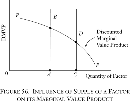
The line PP is the curve of the marginal value product (or discounted MVP) of a factor. It is always declining as it moves to the right, because new units of supply always enter those uses that are most productive of revenue. On the horizontal axis is the quantity of supply of the factor. When the supply is 0A, then the MVP is AB. When the supply is larger at 0C, then the MVP is lower at CD.

Let us say that there are 30 units of factor X available in the economy, and that the MVP corresponding to such a supply is 10 ounces. The price of the 30th unit, then, will tend to be 10 ounces and will be 10 ounces in the ERE. This follows from the tendency of the price of a factor to be equal to its MVP. But now we must recall that there takes place the inexorable tendency in the market for the price of all units of any good to be uniform throughout its market. This must apply to a productive factor just as to any other good. Indeed, this result follows from the very basic law of utility that we have been considering. For, since factor units by definition are interchangeable, the value of one unit will be equal to the value of every other unit at any one time. The value of every unit of a good will be equal to the value of the lowest-ranking use now served by a unit. In the present case, every unit of the factor will be priced at 10 gold ounces.

Suppose, for example, that the owner of the factor unit serving the top-ranking use in our array should demand that he receive 24 ounces, instead of 10 ounces, as his price. In that case, the capitalist in that line of production can refuse to hire this factor and instead bid away the unit employed in the lowest-ranking use, say by paying for the latter 10.5 ounces. The only alternative left to the owner of the factor who had demanded 24 ounces is to replace the other factor in the lowest-ranking spot, at 10 ounces. Effectively, all factors will shift until the prices that they can attain will be uniform throughout the market for their services.

The price of X, then, is determined at 10 ounces. It is determined by the MVP (or rather the DMVP) of the supply, which decreases as the supply increases, and vice versa. Let us assume that Y is also a nonspecific factor and that Z is a factor specific to the particular process considered above. Let us further assume that, by a similar process, the DMVP, and therefore the price, of Y is determined at two ounces.

At this point, we must reintroduce the concept of production within each line. We have been discussing MVPs of factors shifted from one use to another. In our example, a unit of X may have an MVP (or DMVP) of 20 ounces in a particular use; yet its price, as determined by the MVP of the lowest-ranking use for which it is employed, is 10 ounces. This means that, in this use, the capitalist is hiring a factor for 10 ounces which earns for him 20 ounces. Spurred on by this profit, he will hire more units of the factor until the MVP in this use will equal the MVP in the lowest-ranking use, i.e., the factor price, 10 ounces. The same process will occur in regard to each of the other uses. The tendency will always be, then (and this will always obtain in the ERE), for the DMVP of any factor to be equal in each line of production. We will see shortly why increased purchase of a factor even within each line will lower the MVP in that line.

Suppose, then, that the prices of X and Y are 10 and two ounces respectively and that all the capitalists have so arranged their production as to equate the DMVP of each factor in each line with this price. Suppose, further, that the equilibrium point in this particular use is the combination:

3X + 10Y + 2Z → 80 oz.

Substituting the given prices of X and Y:

3 + 20 + 2Z → 80 oz.
               2Z → 80 oz.
                 Z → 80 oz.

Therefore, Z = 15 oz.

The price of the specific factor Z, residual to the other factors, is thereby determined at 15 ounces.

It is obvious that the impact of a change in consumer demand on a specific factor will be far greater, in either direction, than it will be on the price of employment of a nonspecific factor.

It is now clear why the temptation in factor-price analysis is for the firm to consider that factor prices are given externally to itself and that it simply varies its production in accordance with these prices. However, from an analytic standpoint, it should be evident that the array of MVPs as a whole is the determining factor, and the lowest-ranking process in terms of MVP will, through the medium of factor prices, transmit its message, so to speak, to the various firms, each of which will use the factor to such an extent that its DMVP will be brought into alignment with its price. But the ultimate determining factor is the DMVP schedule, not the factor price. To make the distinction, we may term the full array of all MVPs for a factor, the general DMVP schedule of a factor, while the special array of DMVPs within any particular production process or stage, we may term the particular DMVP schedule of the factor. It is the general DMVP schedule that determines the price of the supply of the factor, and then the particular DMVP schedules within each production process are brought into alignment so that the DMVPs of the factor equal its price. Figure 56 above was a general schedule. The particular MVPs are subarrays within the widest array of all the possible alternatives—the general MVP schedule.

In short, the prices of productive factors are determined as follows: Where a factor is isolable, its price will tend toward its discounted marginal value product and will equal its DMVP in the ERE. A factor will be isolable where it is nonspecific, i.e., is useful in more than one productive process, or where it is the only specific factor in a process. The nonspecific factor’s price will be set equal to its DMVP as determined by its general DMVP schedule: the full possible array of DMVPs, given various units of supply of the factor in the economy. Since the most value-productive uses will be chosen first, and the least abandoned first, the curve of general MVP declines as the supply increases. The various particular MVPs in the various processes will be arranged so as to equal the factor price set by the general DMVP schedule. The specific factor’s imputed DMVP is the residual difference between the price of the product and the sum of the prices of the nonspecific factors.

The marginal utility of a unit of a good is determined by a man’s diminishing marginal utility schedule evaluating a certain supply or stock of that good. Similarly, the market’s establishment of the price of a consumers’ good is determined by the aggregate consumer demand schedules—diminishing—and their intersection with the given supply or stock of a good. We are now engaged in pursuing the problem still further and in finding the answer to two general questions: What determines the prices of factors of production on the market, and what determines the quantity of goods that will be produced? We have seen in this section that the price of a factor is determined by its diminishing general (discounted) marginal value productivity curve intersecting with the given supply (stock) of the factor in the economy.

• 1The mathematical bent toward replacing the concepts of cause and effect by mutual determination has contributed to the willingness to engage in circular reasoning. See Rothbard, “Toward a Reconstruction of Utility and Welfare Economics,” p. 236; and Kauder, “Intellectual and Political Roots of the Older Austrian School.”
• 2Clearly, the longer the period of time, the more variable will factor proportions tend to be. Technologically, varying amounts of time are needed to rearrange the various factors.
• 3This justifies the conclusion of Mises, Human Action, p. 336, as compared, for example, with the analysis in George J. Stigler’s Production and Distribution Theories. Mises adds the important proviso that if the factors have the same fixed proportions in all the processes for which they are nonspecific, then here too only bargaining can determine their prices.
• 4Strictly, we should be dealing with discounted MVPs here, but treating just MVPs at this stage merely simplifies matters.
• 5We are here postulating that equal quantities of factors produce equal quantities of results. The famous question whether this condition actually holds (sometimes phrased in pretentious mathematical language as whether the “production function is linear and homogeneous”) is easily resolved if we realize that the proposition: equal causes produce equal results, is the major technological axiom in nature. Any cases that appear to confute this rule only do so in appearance; in reality, supposed exceptions always involve some “indivisibility” where one factor, in effect, cannot change proportionately with other factors.