3. Entrepreneurship and Income
3. Entrepreneurship and Income
A. Costs to the Firm
A. Costs to the Firm
We have seen the basis on which the prices of the factors of production and the interest rate are determined. Looked at from the point of view of an individual entrepreneur, payments to factors are money costs. It is clear that we cannot simply rest on the old classical law that prices of products tend, in the long run, to be equal to their costs of production. Costs are not fixed by some Invisible Hand, but are determined precisely by the total force of entrepreneurial demand for factors of production. Basically, as Böhm-Bawerk and the Austrians pointed out, costs conform to prices, and not vice versa. Confusion may arise because, looked at from the point of view of the individual firm rather than of the economist, it appears as if costs (at least in the sense of the prices of factors) are somehow given, and beyond one’s control.28 If a firm can command a selling price that will more than cover its costs, it remains in business; if not, it will have to leave. The illusion of externally determined costs is prevalent because, as we shall presently see, most factors can be employed in a wide variety of firms, if not industries. If we take the broader view of the economist, however, the various “costs,” i.e., prices of factors, determined by their various DMVPs in alternative uses, are ultimately determined solely by consumers’ demand for all uses. It must not be forgotten, furthermore, that changes in demand and selling price will change the prices and incomes of specialized factors in the same direction. The “cost curves” so fashionable in current economics assume fixed factor prices, thereby ignoring their variability, even for the single firm.
It might be noted that, in this work, there is none of that plethora and tangle of “cost curves” which fill the horizon of almost every recent “neoclassical” work in economics.29 This omission has been deliberate, since it is our contention that the cost curves are at best redundant (thus violating the simplicity principle of Occam’s Razor), and at worst misleading and erroneous.
As an explanation of the pricing of factors and the allocation of output it is obvious that cost curves add nothing new to discussion in terms of marginal productivity. At best, the two are reversible. This can be clearly seen in such texts as E.T. Weiler’s The Economic System and George J. Stigler’s Theory of Price.30 But, in addition, the shift brings with it many grave deficiencies and errors. This is revealed in the very passage in which Stigler explains the reasons for his switch from a perfunctory discussion of productivity to a lengthy treatment of cost curves:
The law of variable proportions has now been explored sufficiently to permit a transition to the cost curves of the individual firm. The fundamentally new element in the discussion will, of course, be the introduction of prices of the productive services. The transition is made here only for the case of competition—that is, the prices of the productive services are constant because the firm does not buy enough of any service to affect its price.31
But by introducing given prices of productive services, the contemporary theorist really abandons any attempt to explain these prices. This is one of the cardinal errors of the currently fashionable theory of the firm. It is highly superficial. One of the aspects of this superficiality is the assumption that prices of productive services are given, without any attempt to explain them. To furnish an explanation, marginal productivity analysis is necessary.
Marginal productivity analysis and the profit motive are sufficient to explain the prices of productive factors and their allocation to various firms and industries in the economy. Furthermore, there are in production theory two important and interesting concepts involving periods of time. One is what we may call the “immediate run”—the market prices of commodities and factors on the basis of given stocks and speculative demands and given consumer valuations. The immediate run is important, since it provides an explanation of the actual market prices of all goods at any time. The other important concept is that of the “final price,” or the long-run equilibrium price, i.e., the price that would be established in the ERE. This is important because it reveals the direction in which the immediate-run market prices tend to move. It also permits the analytic isolation of interest, as compared to profit and loss, in entrepreneurial incomes. In the ERE all factors will receive their discounted marginal value product, and interest will be pure time preference; there will be no profit and loss.
The interesting phases, then, are the immediate run and the long run. Yet cost-curve analysis deals almost exclusively with a hybrid intermediate phase known as the “short run.” In this short run, “costs” are sharply divided into two categories: fixed (which must be incurred regardless of the amount produced) and variable (which vary with output). This whole construction is a highly artificial one. There is no actual “fixity” of costs. Any alleged fixity depends purely on the length of time involved. In fact, suppose that production is zero. The “cost-curve theorists” would have us believe that even at zero output there are fixed costs that must be incurred: rent of land, payment of management, etc. However, it is clear that if data are frozen—as they should be in such an analysis—and the entrepreneurs expect a situation of zero output to continue indefinitely, these “fixed” costs would become “variable” and disappear very quickly. The rent contract for land would be terminated, and management fired, as the firm closed its doors.
There are no “fixed” costs; rather there are different degrees of variability for different productive factors. Some factors are best used in a certain quantity over a certain range of output, while others yield best results over other ranges of output. The result is not a dichotomy into “fixed” and “variable” costs, but a condition of many degrees of variability for the various factors.32
Even if none of these difficulties existed, it is hard to see why the “short run” should be picked out for detailed analysis, when it is merely one way station, or rather a series of way stations, between the important periods of time: the immediate run and the long run. Analytically, the cost-curve approach is at best of little interest.33
With these caveats, let us now turn to an analysis of the costs of the firm. Let us consider what will happen to costs at alternate hypothetical levels of output. There are two elements that determine the behavior of average costs, i.e., total costs per unit output.
(a) There are “physical costs”—the amounts of factors that must be purchased in order to obtain a certain physical quantity of output. These are the obverse of “physical productivity”— the amounts of the physical product that can be produced with various amounts of factors. This is a technological problem. Here the question is not marginal productivity, where one factor is varied while others remain constant in quantity. Here we concentrate on the scale of output when all factors are permitted to vary. Where all factors and the product are completely divisible, a proportionate increase in the quantities of all the factors must lead to an equally proportionate increase in physical output.34 This may be called the law of “constant returns to scale.”
(b) The second determinant of average costs is factor prices. “Pure competition” theorists assume that these prices remain unchanged with a changing scale of output, but this is impossible.35 As any firm’s scale of output increases, it necessarily bids factors of production away from other firms, raising their prices in the process. And this is particularly true for labor and land factors, which cannot be increased in supply via new production. The increase in factor prices as output increases, combined with constant physical costs, raises the average money cost per unit output. We may therefore conclude that if factors and product were perfectly divisible, average cost would always be increasing.
In the productive world, perfect divisibility does not always, or even usually, obtain. Units of factors and of output are indivisible, i.e., they are not purely divisible into very small units. First, the product may be indivisible. Thus, suppose that three units of factor A + 2 units of factor B may combine to produce one refrigerator. Now it may be true that 6A + 4B will produce two refrigerators, according to our law of returns to scale. But it is also true that 4A + 3B will not produce one-and-a-fraction refrigerators. There are bound to be gaps where an increased supply of factors will not lead to an increased product, because of the technological indivisibility of the unit product.
In the areas of the gaps, average costs increase rapidly, since new factors are being hired with no product forthcoming; then, when expenditures on factors are increased sufficiently to produce more of the product, there is a precipitate decline in average cost compared to the situation during the gap. As a result, no businessman will knowingly invest in the area of the gaps. To invest more without yielding a product is sheer waste, and so businessmen will invest only in the trough points outside the gap areas.36
Secondly, and more important, the productive factors may be indivisible. Because of this indivisibility, it is not possible simply to double or halve the quantities of input of every one of the productive services simultaneously. Each factor has its own technological unit size. As a result, almost all business decisions take place in zones in which many factors have to remain constant while others (the more divisible ones) may vary. And these relative divisibilities and indivisibilities are due, not to variations in periods of time, but to the technological size of the various units. In any productive operation there will be many varieties of indivisibility.
Professor Stigler presents the example of a railroad track, a factor capable of handling up to 200 trains a day.37 The track is most efficiently utilized when train runs total precisely 200 a day. This is the technologically “ideal” output and may be the one for which the track was designed. Now what happens when output is below 200? Suppose output is only 100 per day. The divisible factors of production will then be cut in half by the owners of the railroad. Thus, if engineers are divisible, the railroad will hire half as many engineers or hire its engineers for half their usual number of hours. But (and this is the critical point here) the railroad cannot cut the track in half and operate on half a track. The technological unit of “track” being what it is, the number of tracks has to remain at one. Conversely, when output increases to 200 again, other productive services may be doubled, but the quantity of track remains the same.38
What happens should output increase to 250 trains a day—a 25-percent increase over the planned quantity? Divisible services such as engineers may be increased by one-fourth; but the track must either remain at one—and be overutilized—or be increased to two. If it is increased, the tracks will again be underutilized at 250, because the “ideal” output from the point of view of utilizing the tracks is now 400.
When an important indivisible factor is becoming less and less underutilized, the tendency will be for “increasing returns,” for decreasing average costs as output increases. When an important indivisible factor is becoming more and more overutilized, there is a tendency for increasing average costs.
In some spheres of production, indivisibilities may be such that full utilization of one indivisible factor requires full utilization of all.39 In that case, all the indivisible factors move together and can be lumped together for our purposes; they become the equivalent of one indivisible factor, such as the railroad track. In such cases again, average costs will first decline with an increase in output, as the increased output remedies an underutilization of the lumped indivisible factors. After the technologically most efficient point is reached, however, costs will increase, given the indivisible factors. The tendency for costs to decline will, in addition, be offset by the rise in factor prices caused by the increase in output.
In the overwhelming majority of cases, however, each factor will differ from the others in size and degree of divisibility. As a consequence, any size or combination chosen might utilize one indivisible factor most efficiently, but at the expense of not utilizing some other indivisible factor at peak efficiency. Suppose we consider a hypothetical schedule of average money cost at each alternative output. When we start at a very low level of output, all the indivisible factors will be underutilized. Then, as we expand production, average costs will decrease unless offset by the price rise for those divisible factors needed to expand production. As soon as one of the indivisible factors is fully utilized and becomes overworked, average costs will rise sharply. Later, a tendency toward decreasing costs sets in again as another underutilized factor becomes more fully utilized. The result is an alternating series of decreases and increases in average costs as output increases. Eventually, a point will be reached at which more indivisible factors will be overutilized than underutilized, and from then on the general trend of average cost as output increases will be upward. Before that point, the trend will be downward.
Mingling with these influences from the technological side of costs are the continuing rises in factor prices, which also become more important as output increases.
In sum, as Mises states:
Other things being equal, the more the production of a certain article increases, the more factors of production must be withdrawn from other employments in which they would have been used for the production of other articles. Hence—other things being equal—average production costs increase with the increase in the quantity produced. But this general law is by sections superseded by the phenomenon that not all factors of production are perfectly divisible and that, as far as they can be divided, they are not divisible in such a way that full utilization of one of them results in full utilization of the other imperfectly divisible factors.40
Some indivisible factors, such as the railroad track, can be available in only one particular size. Other indivisible factors, such as machinery, can be built in various sizes. Cannot a small factory, then, use small-scale machinery which will be just as efficient as large-scale machinery in a larger factory, and would this not eliminate indivisibilities and result in constant costs? No, for here too, one particular size will probably be most efficient. Below the most efficient size, operating the machine will be more costly. Thus, as Stigler says, “fitting together of the parts of a ten-horsepower motor does not require ten times the labor necessary to fit those of a one-horsepower motor. Similarly, a truck requires one driver, whether it has a half-ton or two-ton capacity.”41
It is also true that an oversized machine will be more costly than the optimum. But this will be no limitation on the size of the firm, for a large firm can simply use several (smaller) optimum-sized machines instead of one huge machine.
Labor is usually treated as a perfectly divisible factor, as one that varies directly with the size of the output. But this is not true. As we have seen, the truck driver is not divisible into fractions. Further, management tends to be an indivisible production factor. So also salesmen, advertising, cost of borrowing, research expenditures, and even insurance for actuarial risk. There are certain basic costs in borrowing which simply arise from investigating, paperwork, etc. These will tend to be proportionately smaller the larger the size—another indivisibility, with returns increasing over a certain area. Also, the broader the coverage, the lower insurance premiums will be.42
Then there are the well-known gains from the increase in the division of labor with larger outputs. The benefits from the division of labor may be considered indivisible. They arise from the specialized machines that must first be used with a larger product, and similarly from the increased labor skills of specialists. Here too, however, there is a point beyond which no further specialization is possible or where specialization is subject to increasing costs. Management has usually been stressed as particularly subject to overutilization. Even more important is the factor of ultimate-decision-making ability, which cannot be enlarged to the extent that management can.
What any given firm’s size and output will be is therefore subject to a host of conflicting determinants, some impelling a limitation, some an expansion, of size. At what point any firm will settle depends on the concrete data of the actual case and cannot be decided by economic analysis. Only the actual entrepreneur, through the give and take of the market, can decide where the maximum-profit size is and can set the firm at that point. This is the task of the businessman and not of the economist.43
Furthermore, the cost-curve diagrams, so simple and smooth in the textbooks, misinterpret real conditions. We have seen that there are a whole host of determinants which tend at any point toward increasing and toward decreasing costs. It is, of course, true that an entrepreneur will seek to produce at the point of maximum profit, i.e., of maximum net returns over costs. But the factors that influence his decision are too numerous and their interactions too complex to be captured in cost-curve diagrams.
It is clear to almost everyone that the optimum size of a firm in some industries is larger than in others. The economic optimum for a steel plant is larger than the optimum barbershop. In industries where large-scale firms have demonstrated the most efficiency, however, many people have worried a great deal about an alleged tendency for decreasing costs to continue permanently and therefore for “monopoly” to result from ever-larger firms. It should be obvious, however, that there is no infinite tendency for ever-larger size; this is clear from the very fact that every firm, at any time, always has a finite size and that, therefore, an economic limit must have been imposed upon it from some direction. Furthermore, we have seen that the general rule of operating in a zone of diminishing marginal productivity for each factor, as well as the tendency for product prices to decline and factor prices to increase as output increases, establishes limits on the size of each firm. And, as a neglected point, we shall see that ultimate limits are set on the relative size of the firm by the necessity for markets to exist in every factor, in order to make it possible for the firm to calculate its profits and losses.44
Money costs will equal opportunity costs to the businessman only when he plans an investment in factors. To the extent that his money costs are “sunk” in any production process, they are committed irrevocably, and any future plans must consider them as irretrievably spent.45 The businessman’s market-supply curve will depend on his present opportunity cost, not his past money cost. For the businessman sells his goods at any price that will more than cover any further costs that must be incurred in selling them. As capital goods move toward final output in any stage of the production structure, more and more investment has been sunk into the process. Therefore, the marginal cost of further production (roughly the opportunity cost) becomes ever lower as the product moves toward final output and sale. This is the simple meaning of the usual cost-curve morass. When, for example, some costs are not “fixed,” but irrevocable from the point of view of further short-run production, they are not included in the businessman’s estimated costs of such further production. As we have seen above, the sale of immediate stock completely ready for sale is virtually “costless,” since there are no further costs for its production—in the immediate run.46 In the ERE, of course, all costs and investments will be adjusted, and irrevocably incurred costs will present no problem. In the ERE average money costs for all firms will equal the price of the product minus pure interest return to the capitalist-entrepreneurs, and also, as we shall see, minus the return to the “discounted marginal productivity of the owner,” a factor which does not enter into the firm’s money costs.47 ,48
- 28Hence, when the economist considers only the single firm (as in recent years), he goes completely astray by ignoring the generality of economic interrelations. To analyze means-ends relations logically, as economics does, requires taking all relations into account. Failure to do so, either by treating the single firm only or by treating unreal holistic aggregates or by taking refuge in the irrelevant mathematics of the Lausanne “general equilibrium” school, is equivalent to abandoning economics.
- 29Many beginning students come away with the impression that economics consists of an indigestible brew of “cost curves” to be memorized by rote and drawn neatly on the blackboard.
- 30E.T. Weiler, The Economic System (New York: Macmillan & Co., 1952), pp. 141–61; Stigler, Theory of Price, pp. 126ff.
- 31Stigler, Theory of Price, p. 126.
- 32Robbins points out that the length of a period of productive activity depends upon the expectations of entrepreneurs concerning the permanence of a change and the technical obstacles to a change. Robbins, “Remarks upon Certain Aspects of the Theory of Costs,” pp. 17–18.
- 33For a critique of cost-curve theory, see the articles by Robbins, Thirlby, and Gabor and Pearce cited above, especially Gabor and Pearce, “A New Approach to the Theory of the Firm.” Also see Milton Friedman, “Survey of the Empirical Evidence on Economies of Scale: Comment” in Business Concentration and Price Policy (Princeton, N.J.: National Bureau of Economic Research, 1955), pp. 230–38; Armen Alchian, “Costs and Outputs” in The Allocation of Economic Resources (Stanford: Stanford University Press, 1959), pp. 23–40; F.A. Hayek, “Unions, Inflation, and Prices” in Philip D. Bradley, ed., The Public Stake in Union Power (Charlottesville: University of Virginia Press, 1959), pp. 55 f.; Hayek, Pure Theory of Capital, pp. 14, 20–21; Harrod, “Theory of Imperfect Competition Revised” in Economic Essays, pp. 139–87; G. Warren Nutter, “Competition: Direct and Devious,” American Economic Review, Papers and Proceedings, May, 1954, pp. 69ff.; Scott, Natural Resources: The Economics of Conservation, p. 5.
- 34This law follows from the natural law that every quantitatively observable cause-effect relation can be duplicated. For example, if x + 2y + 3em>z are necessary and sufficient to form 1p, another set will form another p, so that 2x + 4y + 6z will yield 2p.
- 35See chapter 10 for more on the theory of pure competition.
- 36For example, suppose that 1,000 gold ounces invested in factors yield 100 units of product and that 1,100 ounces yield 101 units. All the points in the gap between 1,000 and 1,100 will yield no more than 100 units. The excess of investment over 1,000 and under 1,100 ounces is clearly sheer waste, and no businessman will invest within the gap. Instead, investments will be made at such trough points for average cost as 1,000 and 1,100.
- 37Stigler, Theory of Price, pp. 132ff.
- 38We are not discussing the fact that the railroad could, of course, cut down or increase the mileage of its track by including less or more geographic area in its service. The example assumes a given geographic area in which the railroad operates.
- 39See Mises, Human Action, pp. 338–40. This is the unrealistic condition implicitly assumed by textbook “cost curves.”
- 40Ibid., p. 340.
- 41Stigler, Theory of Price, p. 136.
- 42It is particularly important not to limit possible efficiencies from large-scale production to narrow technological factors such as the “size of the plant.” There are also efficiencies derived from the organization of a firm owning several plants—e.g., management utilization, specialization, efficiency of large-scale purchasing and selling, research expenditures, etc. Cf. George G. Hagedorn, Studies on Concentration (New York: National Association of Manufacturers, 1951), pp. 14 ff.
- 43See Friedman, “Survey of the Empirical Evidence on Economies of Scale: Comment,” pp. 230–38.
- 44For a good, largely empirical, study of size of firm, see George G. Hagedorn, Business Size and the Public Interest (New York: National Association of Manufacturers, 1949). Also see idem, Studies on Concentration, and John G. McLean and Robert W. Haigh, “How Business Corporations Grow,” Harvard Business Review, November–December, 1954, pp. 81–93.
- 45Plans are relevant, not only in the ERE, but also to all decisions on maintenance or replacement, as well as additions to capital goods when they wear out or fall into disrepair.
- 46It is costless only if no rise in the price of the good is foreseen for the near future. If it is, then there will arise the opportunity cost of forgoing a higher price. Hence, if there is no hope of a higher price, the businessman will sell, however low the price (adjusting for the costs of selling minus the costs of continued storage).
- 47Conventional “cost-curve” analysis depicts average cost and demand curves as tangential in the ERE—i.e., that price = average cost. But (aside from the unreality of assuming smooth curves rather than discontinuous angles), interest return—as well as return to the owner’s decision-making ability—will accrue to the entrepreneurs even in the ERE. Hence, no such tangency can arise. See chapter 10 below for the implications of this revision for “monopolistic competition” theory.
- 48For further readings on cost, see G.F. Thirlby, “The Marginal Cost Controversy: A Note on Mr. Coase’s Model,” Economica, February, 1947, pp. 48–53; F.A. Fetter’s classic “The Passing of the Old Rent Concept,” p. 439; R.H. Coase, “Business Organization and the Accountant,” The Accountant, October l–November 26, 1938; and idem, “Full Costs, Cost Changes, and Prices” in Business Concentration and Price Policy, pp. 392–94; John E. Hodges, “Some Economic Implications of Cost-Plus Pricing,” Southwestern Social Science Quarterly, December, 1954, pp. 225–34; I.F. Pearce, “A Study in Price Policy,” Economica, May, 1956, pp. 114–27; I.F. Pearce and Lloyd R. Amey, “Price Policy with a Branded Product,” Review of Economic Studies, Vol. XXIV (1956–57), No. 1, pp. 49–60; James S. Earley, “Recent Developments in Cost Accounting and the ‘Marginal Analysis’ ,” Journal of Political Economy, June, 1955, pp. 227–42; and David Green, Jr., “A Moral to the Direct-Costing Controversy,” Journal of Business, July, 1960, pp. 218–26.
B. Business Income
B. Business Income
The net incomes in the economy accrue to labor in wages, to landowners in ground rents (both wages and ground rents being “rents,” i.e., unit-prices of productive factors), to capitalists in interest—all of which continue in the ERE—and profits and losses to entrepreneurs, which do not. (Ground rents are capitalized in the capital value of land, which therefore earns the interest rate in the ERE.) But what of the owners? Are their incomes exhausted by the category of entrepreneurial profit and loss, which we have studied in chapter 8, or will they continue to earn income beyond interest in the ERE?
So far we have seen that owners of businesses perform an entrepreneurial function: the function of uncertainty-bearing in an ever-changing world. Owners are also capitalists, who advance present funds to labor and land factors and earn interest. They may also be their own managers; in that case, they earn an implicit wage of management, since they are performing work which could also be performed by employees.49 We have seen that, catallactically, labor is the personal energy of nonowners in production, and that this factor receives wages. When the owner does laboring work himself, then he too earns an implicit wage. This wage, of course, continues also in the ERE.
But is there a function which owning businessmen perform, and would still perform in the ERE, beyond the advancing of capital or possible managerial work? The answer is that they do execute another function for which they cannot hire other factors. It goes beyond the simple capital-advancing function, and it still continues in the ERE. For want of a better term, it may be called the decision-making function, or the ownership function. Hired managers may successfully direct production or choose production processes. But the ultimate responsibility and control of production rests inevitably with the owner, with the businessman whose property the product is until it is sold. It is the owners who make the decision concerning how much capital to invest and in what particular processes. And particularly, it is the owners who must choose the managers. The ultimate decisions concerning the use of their property and the choice of the men to manage it must therefore be made by the owners and by no one else. It is a function necessary to production, and one that continues in the ERE, since even in the ERE there are skills needed to hire proper managers and invest in the most efficient processes; and even though these skills remain constant, the efficiency with which they are performed will differ from one firm to another, and differing returns will be received accordingly.50
The decision-making factor is necessarily specific to each firm. We cannot call what it earns a wage because it can never be hired, and thus it does not earn an implicit wage. We may therefore call the income of this factor, the “rent of decision-making ability.”51 It is clear that this rent will be equal to the factor’s DMVP, the amount which it specifically contributes to the firm’s revenue. Since this ability differs from one owner to the next, the rents will differ accordingly. This difference accounts for the phenomena of “high-cost” and “low-cost” firms in any industry and indicates that differences in efficiency among firms are not solely functions of ephemeral uncertainty, but would persist even in the ERE.
Granting that the “supramarginal” (i.e., the lower-cost) firms in an industry are earning rents of decision-making ability for their owners, what of the “marginal” firms in the industry, the “high-cost” firms just barely in business? Are their owners earning rents of decision-making ability? Many economists have believed that these marginal firms earn no such income, just as they have believed that the marginal land earns zero rent. We have seen, however, that the marginal land earns some rent, even if “close to” zero. Similarly, the marginal firm earns some rent of decision-making ability. We can never say quantitatively how much it will be, only that it will be less than the corresponding “decision rents” of the supramarginal firms.
The belief that marginal firms earn no decision rents whatever seems to stem from two errors: (1) the assumption of mathematical continuity, so that successive points blend together; and (2) the assumption that “rent” is basically differential and therefore that the most inferior working land or firm must earn zero to establish the differential. We have seen, however, that rents are “absolute”—the earnings and marginal value products of factors. There is no necessity, therefore, for the poorest factor to earn zero, as we can see when we realize that wages are a subdivision of rents and that there is clearly no one making a zero wage. And so neither does the marginal firm earn a decision rent of zero.
That the decision rent earned by the marginal firm must be positive and not zero becomes evident if we consider a firm whose decision rent is only zero. Its owner would then be performing certain functions—making and bearing responsibility for ultimate decisions about his property and choosing the top managers—and yet receiving no return. And this in the ERE, where it cannot be simply the unforeseen result of entrepreneurial mistakes! But there will be no reason for the owner to continue performing these functions without a return. He will not continue to earn what is psychically a negative return, for while he remained in business he would continue to expend energy in ownership while receiving nothing in return.
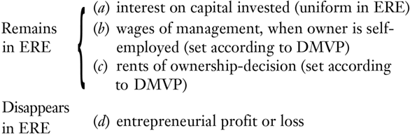
To sum up, the income accruing to a business owner, in a changing economy, will be a composite of four elements:
We have, so far, been dealing almost exclusively with capitalist-entrepreneurs. Since the entrepreneur is the actor in relation to natural uncertainty, the capital investor, who hires and makes advances to other factors, plays a peculiarly important entrepreneurial role. Making decisions concerning how much and where to invest, he is the driving force of the modern economy. Laborers are also entrepreneurs in the sense of predicting demand in the markets for labor and choosing to enter certain markets accordingly. Someone who emigrates from one country to another in expectation of a higher wage is in this sense an entrepreneur and may obtain a monetary profit or loss from his move. One important distinction between capitalist-entrepreneurs and laborer-entrepreneurs is that only the former may suffer negative incomes in production. Even if a laborer emigrates to a nation where pay turns out to be lower than expected, he absorbs only a differential, or “opportunity,” loss from what he might have earned elsewhere. But he still earns a positive wage in production. Even in the unlikely event of a labor surplus vis-à-vis land, the laborer earns zero and not negative wages. But the capitalist-entrepreneur, the man who hires the other factors, can and does incur actual monetary losses from his entrepreneurial effort.
- 49This implicit wage will equal the DMVP of the owner’s managerial services, which will tend to equal the “opportunity wage forgone” that he could be earning as a manager elsewhere.
- 50In one of those extremely fertile but neglected hints of his, Böhm-Bawerk wrote:
But even where he [the businessman] does not personally take part in the carrying out of the production, he yet contributes a certain amount of personal trouble in the shape of intellectual superintendence—say, in planning the business, or, at the least, in the act of will by which he devotes his means of production to a definite undertaking. (Böhm-Bawerk, Capital and Interest, p. 8) - 51For an interesting contribution to the theory of business income, though not coinciding with the one presented here, see Harrod, “Theory of Profit” in Economic Essays, pp. 190–95. Also see Friedman, “Survey of the Empirical Evidence on Economies of Scale: Comment.”
C. Personal Consumer Service
C. Personal Consumer Service
A particularly important category of laborer-entrepreneurs is that of the sellers of personal services to consumers. These laborers are generally capitalists as well. The sellers of such services—doctors, lawyers, concert artists, servants, etc.—are self-employed businessmen, who, in addition to interest on whatever capital they have invested, earn an implicit “managerial” wage for their labor.52 ,53 Thus, they earn a peculiar type of income: a business return consisting almost exclusively of labor income. We may call this type of work direct labor, since it is labor that serves directly as a consumers’ good rather than hired as a factor of production. And since it is a consumers’ good, this labor service is priced directly on the market.
The determination of the prices of these goods will be similar on the demand side to that of any consumers’ good. Consumers evaluate marginal units of the service on their value scales and decide how much, if any, to purchase. There is a difference, however, on the supply side. The market-supply curves for most consumers’ goods are vertical straight lines, since the sale of the product, once produced, is costless to the entrepreneur. He has no alternative use for it. The case of personal service, however, is different. In the first place, leisure is a definite alternative to work. In the second place, as a result of the connexity of the labor market, the worker can shift to a higher-paying occupation further up on the structure of production if his income in this occupation is unsatisfactory. As a result, for this type of consumers’ good, the supply curve is likely to be a rather flat, forward-sloping one.
The seller of the service, or the direct laborer, earns, as do all factors, his DMVP to the consumer. He will allocate his labor to whatever branch, whether high or low in the structure of production, where his DMVP will be the highest, and where, as a consequence, his wage rate will be the greatest. The principles of allocation, then, between direct labor and indirect labor in production are the same as those among the various branches of indirect productive use.
- 52Since the scope of their business property and decisions is relatively negligible compared to their labor services, we may neglect their decision rents here.
- 53It is a managerial wage, even though the only employee may be the owner himself. It may seem strange to classify a domestic servant as “self-employed,” but actually he is no different from a doctor or a lawyer to the extent that the latter sells his services to consumers rather than to capitalists.
D. Market Calculation and Implicit Earnings
D. Market Calculation and Implicit Earnings
We have seen that a musician or a doctor earns wages without being an employee; the wages of each are implicit in the income that he receives, even though they are received directly from the consumers.
In the real world, each function is not necessarily performed by a different person. The same person can be a landowner and a worker. Similarly, a particular firm, or rather its owner or owners, may own land and participate in the production of capital goods. The owner may also manage his own firm. In practice, the different sources of income can be separated only by referring to these incomes as determined by prices on the market. For example, suppose that a man owns a firm which invests its capital, owns its own ground land, and produces a capital good, and that he manages the plant himself. He receives a net income over a year’s period of 1,000 gold ounces. How can he estimate the different sources of his income? Suppose that he had invested 5,000 gold ounces in the business. He looks around at the economy and finds that what he can pretty well call the ruling rate of interest, toward which the economy is tending, is 5 percent. He then concludes that 250 gold ounces of his net income was implicit interest. Next, he estimates approximately what he would have received in wages of management if he had gone to work for a competing firm rather than engaging in this business. Suppose he estimates that this would have been 500 gold ounces. He then looks to his ground land. What could he have received for the land if he had rented it out instead of using it himself in the business? Let us say that he could have received 400 ounces in rental income for the land.
Now, our owner received a net money income, as landowner-capitalist-laborer-entrepreneur, of 1,000 gold ounces for the year. He then estimates what his costs were, in money terms. These costs are not his explicit money expenses, which have already been deducted to find his net income, but his implicit expenses, i.e., his opportunities forgone by engaging in the business. Adding up these costs, he finds that they total:

Thus, the entrepreneur suffered a loss of 150 ounces over the period. If his opportunity costs had been less than 1,000, he would have gained an entrepreneurial profit.
It is true that such estimates are not precise. The estimates of what he would have received can never be wholly accurate. But this tool of ex post calculation is an indispensable one. It is the only way by which a man can guide his ex ante decisions, his future actions. By means of this calculation, he may realize that he is suffering a loss in this business. If the loss continues much longer, he will be impelled to shift his various resources to other lines of production. It is only by means of such estimates that an owner of more than one type of factor in the firm can determine his gains or losses in any situation and then allocate his resources to strive for the greatest gains.
A very important aspect of such estimates of implicit incomes has been overlooked: there can be no implicit estimates without an explicit market! When an entrepreneur receives income, in other words, he receives a complex of various functional incomes. To isolate them by calculation, there must be in existence an external market to which the entrepreneur can refer. This is an extremely important point, for, as we shall soon see in detail, this furnishes a most important limitation on the relative potential size of a single firm on the market.
For example, suppose we return for a moment to our old hypothetical example in which each firm is owned jointly by all its factor-owners. In that case, there is no separation at all between workers, landowners, capitalists, and entrepreneurs. There would be no way, then, of separating the wage incomes received from the interest or rent incomes or profits received. And now we finally arrive at the reason why the economy cannot consist completely of such firms (called “producers’ co-operatives”).54 For, without an external market for wage rates, rents, and interest, there would be no rational way for entrepreneurs to allocate factors in accordance with the wishes of the consumers. No one would know where he could allocate his land or his labor to provide the maximum monetary gains. No entrepreneur would know how to arrange factors in their most value-productive combinations to earn the greatest profit. There could be no efficiency in production because the requisite knowledge would be lacking. The productive system would be in complete chaos, and everyone, whether in his capacity as consumer or as producer, would be injured thereby. It is clear that a world of producers’ co-operatives would break down for any economy but the most primitive, because it could not calculate and therefore could not arrange productive factors to meet the desires of the consumers and hence earn the highest incomes for the producers.
- 54Another reason why an economy of producers’ co-operatives could not calculate is that every original factor would be tied indissolubly to a specific line of production. There can be no calculation where all factors are purely specific.
E. Vertical Integration and the Size of the Firm
E. Vertical Integration and the Size of the Firm
In the free economy, there is an explicit time market, labor market, and land-rent market. It is clear that while chaos would ensue from a world of producers’ co-operatives, other critical points even before that would, as it were, introduce little bits of chaos into the productive system. Thus, suppose that workers are separated from capitalists, but that all capitalists own their own ground land. Further, suppose, that for one reason or another, no capitalist will be able to rent out his land to some other firm. In that case, land and a particular capital and production process are indissolubly wedded to each other. There would be no rational way to allocate land in production, since it would have no explicit price anywhere. Since producers would suffer heavy losses, the free market would never establish such a situation. For the free market always tends to conduct affairs so that entrepreneurs make the greatest profit through serving the consumer best and most efficiently. Since absence of calculation creates grave inefficiencies in the system, it also causes heavy losses. Such a situation (absence of calculation) would therefore never be established on a free market, particularly after an advanced economy has already developed calculation and a market.
If this is true for such cases as a world of producers’ co-operatives and the absence of a rent market, it also holds true, on a smaller scale, for “vertical integration” and the size of a firm. Vertical integration occurs when a firm produces not only at one stage of production, but over two or more stages. For example, a firm becomes so large that it buys labor, land, and capital goods of the fifth order, then works on these capital goods, producing other capital goods of the fourth order. In another plant, it then works on the fourth-order capital goods until they become third-order capital goods. It then sells the third-order product.
Vertical integration, of course, lengthens the production period for any firm, i.e., it lengthens the time before the firm can recoup its investment in the production process. The interest return then covers the time for two or more stages rather than one.55 There is a more important question involved, however. This is the role of implicit earnings and calculation in a vertically integrated firm. Let us take the case of the integrated firm mentioned in Figure 65.

Figure 65 depicts a vertically integrated firm; the arrows represent the movement of goods and services (not of money). The firm buys labor and land factors at both the fifth and the fourth stages; it also makes the fourth-stage capital goods itself and uses them in another plant to make a lower-stage good. This movement internal to the firm is expressed by the dotted arrow.
Does such a firm employ calculation within itself, and if so, how? Yes. The firm assumes that it sells itself the fourth-rank capital good. It separates its net income as a producer of fourth-rank capital from its role as producer of third-rank capital. It calculates the net income for each separate division of its enterprise and allocates resources according to the profit or loss made in each division. It is able to make such an internal calculation only because it can refer to an existing explicit market price for the fourth-stage capital good. In other words, a firm can accurately estimate the profit or loss it makes in a stage of its enterprise only by finding out the implicit price of its internal product, and it can do this only if an external market price for that product is established elsewhere.
To illustrate, suppose that a firm is vertically integrated over two stages, with each stage covering one year’s time. The general rate of interest in the economy tends towards 5 percent (per annum). This particular firm, say, the Jones Manufacturing Company, buys and sells its factors as shown in Figure 66.

This vertically integrated firm buys factors at the fifth rank for 100 ounces and original factors at the fourth rank for 15 ounces; it sells the final product at 140 ounces. It seems that it has made a handsome entrepreneurial profit on its operations, but can it find out which stage or stages is making this profitable showing? If there is an external market for the product of the stage that the firm has vertically integrated (stage 4), the Jones Company is able to calculate the profitability of specific stages of its operations. Suppose, for example, that the price of the fourth-order capital good on the external market is 103 ounces. The Jones Company then estimates its implicit price for this intermediate product at what it would have brought on the market if it had been sold there. This price will be about 103 ounces.56 Assuming that the price is estimated at 103, then the total amount of money spent by Jones’ lower-order plant on factors is 15 (explicit, on original factors) plus 103 (implicit, on capital goods) for a total of 118.
Now the Jones Company can calculate the profits or losses made at each stage of its operations. The “higher” stage bought factors for 100 ounces and “sold” them at 103 ounces. It made a 3-percent return on its investment. The lower stage bought its factors for 118 ounces and sold the product for 140 ounces, making a 29-percent return. It is obvious that, instead of enjoying a general profitability, the Jones Company suffered a 2-percent entrepreneurial loss on its earlier stage and gained a 24-percent profit on its later stage. Knowing this, it will shift resources from the higher to the lower stage in accordance with their respective profitabilities—and therefore in accordance with the desires of consumers. Perhaps it will abandon its higher stage altogether, buying the capital good from an external firm and concentrating its resources in the more profitable lower stage.
On the other hand, suppose that there is no external market, i.e., that the Jones Company is the only producer of the intermediate good. In that case, it would have no way of knowing which stage was being conducted profitably and which not. It would therefore have no way of knowing how to allocate factors to the various stages. There would be no way for it to estimate any implicit price or opportunity cost for the capital good at that particular stage. Any estimate would be completely arbitrary and have no meaningful relation to economic conditions.
In short, if there were no market for a product, and all of its exchanges were internal, there would be no way for a firm or for anyone else to determine a price for the good. A firm can estimate an implicit price when an external market exists; but when a market is absent, the good can have no price, whether implicit or explicit. Any figure could be only an arbitrary symbol. Not being able to calculate a price, the firm could not rationally allocate factors and resources from one stage to another.
Since the free market always tends to establish the most efficient and profitable type of production (whether for type of good, method of production, allocation of factors, or size of firm), we must conclude that complete vertical integration for a capital-good product can never be established on the free market (above the primitive level). For every capital good, there must be a definite market in which firms buy and sell that good. It is obvious that this economic law sets a definite maximum to the relative size of any particular firm on the free market.57 Because of this law, firms cannot merge or cartelize for complete vertical integration of stages or products. Because of this law, there can never be One Big Cartel over the whole economy or mergers until One Big Firm owns all the productive assets in the economy. The force of this law multiplies as the area of the economy increases and as islands of noncalculable chaos swell to the proportions of masses and continents. As the area of incalculability increases, the degrees of irrationality, misallocation, loss, impoverishment, etc., become greater. Under one owner or one cartel for the whole productive system, there would be no possible areas of calculation at all, and therefore complete economic chaos would prevail.58
Economic calculation becomes ever more important as the market economy develops and progresses, as the stages and the complexities of type and variety of capital goods increase. Ever more important for the maintenance of an advanced economy, then, is the preservation of markets for all the capital and other producers’ goods.
Our analysis serves to expand the famous discussion of the possibility of economic calculation under socialism, launched by Professor Ludwig von Mises over 40 years ago.59 Mises, who has had the last as well as the first word in this debate, has demonstrated irrefutably that a socialist economic system cannot calculate, since it lacks a market, and hence lacks prices for producers’ and especially for capital goods.60 Now we see that, paradoxically, the reason why a socialist economy cannot calculate is not specifically because it is socialist! Socialism is that system in which the State forcibly seizes control of all the means of production in the economy. The reason for the impossibility of calculation under socialism is that one agent owns or directs the use of all the resources in the economy. It should be clear that it does not make any difference whether that one agent is the State or one private individual or private cartel. Whichever occurs, there is no possibility of calculation anywhere in the production structure, since production processes would be only internal and without markets. There could be no calculation, and therefore complete economic irrationality and chaos would prevail, whether the single owner is the State or private persons.
The difference between the State and the private case is that our economic law debars people from ever establishing such a system in a free-market society. Far lesser evils prevent entrepreneurs from establishing even islands of incalculability, let alone infinitely compounding such errors by eliminating calculability altogether. But the State does not and cannot follow such guides of profit and loss; its officials are not held back by fear of losses from setting up all-embracing cartels for one or more vertically integrated products. The State is free to embark upon socialism without considering such matters. While there is therefore no possibility of a one-firm economy or even a one-firm vertically integrated product, there is much danger in an attempt at socialism by the State. A further discussion of the State and State intervention will be found in chapter 12 of this book.
A curious legend has become quite popular among the writers on the socialist side of the debate over economic calculation. This runs as follows: Mises, in his original article, asserted “theoretically” that there could be no economic calculation under socialism; Barone proved mathematically that this is false and that calculation is possible; Hayek and Robbins conceded the validity of this proof but then asserted that calculation would not be “practical.” The inference is that the argument of Mises has been disposed of and that all socialism needs is a few practical devices (perhaps calculating machines) or economic advisers to permit calculation and the “counting of the equations.”
This legend is almost completely wrong from start to finish. In the first place, the dichotomy between “theoretical” and “practical” is a false one. In economics, all arguments are theoretical. And, since economics discusses the real world, these theoretical arguments are by their nature “practical” ones as well.
The false dichotomy disposed of, the true nature of the Barone “proof” becomes apparent. It is not so much “theoretical” as irrelevant. The proof-by-listing-of-mathematical-equa-tions is no proof at all. It applies, at best, only to the evenly rotating economy. Obviously, our whole discussion of the calculation problem applies to the real world and to it only. There can be no calculation problem in the ERE because no calculation there is necessary. Obviously, there is no need to calculate profits and losses when all future data are known from the beginning and where there are no profits and losses. In the ERE, the best allocation of resources proceeds automatically. For Barone to demonstrate that the calculation difficulty does not exist in the ERE is not a solution; it is simply a mathematical belaboring of the obvious.61 The difficulty of calculation applies to the real world only.62
- 55Vertical integration, we might note, tends to reduce the demand for money (to “turn over” at various stages) and thereby to lower the purchasing power of the monetary unit. For the effect of vertical integration on the analysis of investment and the production structure, see Hayek, Prices and Production, pp. 62–68.
- 56The implicit price, or opportunity cost of selling to oneself, might be less than the existing market price, since the entry of the Jones Company on the market might have lowered the price of the good, say to 102 ounces. There would be no way at all, however, to estimate the implicit price if there were no external market and external price.
- 57On the size of a firm, see the challenging article by R.H. Coase, “The Nature of the Firm” in George J. Stigler and Kenneth E. Boulding, eds., Readings in Price Theory (Chicago: Richard D. Irwin, 1952), pp. 331–51. In an illuminating passage Coase pointed out that State “planning is imposed on industry, while firms arise voluntarily because they represent a more efficient method of organizing production. In a competitive system there is an ‘optimum’ amount of planning.” Ibid., p. 335 n.
- 58Capital goods are stressed here because they are the product for which the calculability problem becomes important. Consumers’ goods per se are no problem, since there are always many consumers buying goods, and therefore consumers’ goods will always have a market.
- 59See the classic presentation of the position in Ludwig von Mises, “Economic Calculation in the Socialist Commonwealth,” reprinted in F.A. Hayek, ed., Collectivist Economic Planning (London: George Routledge & Sons, 1935), pp. 87–130. Also see in the Hayek volume the other essays by Hayek, Pierson, and Halm. Mises continued his argument in Socialism (2nd ed.; New Haven: Yale University Press, 1951), pp. 135–63, and refutes more recent criticisms in his Human Action, pp. 694–711. Aside from these works, the best book on the subject of economic calculation under socialism is Trygve J.B. Hoff, Economic Calculation in the Socialist Society (London: William Hodge, 1949). Also see F.A. Hayek, “Socialist Calculation III, the Competitive ‘Solution’” in Individualism and the Economic Order, pp. 181–208, and Henry Hazlitt’s remarkable essay in fictional form, The Great Idea (New York: Appleton-Century-Crofts, 1951).
- 60It is remarkable that so many antisocialist writers have never become aware of this critical point.
- 61Far from being refuted, Mises had already disposed of this argument in his original article. See Hayek, Collectivist Economic Planning, p. 109. Further, Barone’s article was written in 1908, 12 years before Mises’. A careful perusal of Mises’ original article, in fact, reveals that he there disposed of almost all the alleged “solutions” which decades later were brought forth as “new” attempts to refute his argument.
- 62Part of the confusion stems from an unfortunate position taken by two followers of Mises in this debate—Hayek and Robbins. They argued that a socialist government could not calculate because it simply could not compute the millions of equations that would be necessary. This left them open to the obvious retort that now, with high-speed computers available to the government, this practical objection is no longer relevant. In reality, the job of rational calculation has nothing to do with computing equations. Nobody has to worry about “equations” in real life except mathematical economists. Cf. Lionel Robbins, The Great Depression (New York: Macmillan & Co., 1934), p. 151, and Hayek in Collectivist Economic Planning, pp. 212f.