2. Determination of the Discounted Marginal Value Product
2. Determination of the Discounted Marginal Value Product
A. Discounting
A. Discounting
If the DMVP schedules determine the prices of nonspecific factor services, what determines the shape and position of the DMVP schedules? In the first place, by definition it is clear that the DMVP schedule is the MVP schedule for that factor discounted. There is no mystery about the discounting; as we have stated, the MVP of the factor is discounted in accordance with the going pure rate of interest on the market. The relation of the MVP schedule and the DMVP schedule may be diagrammed as in Figure 57.
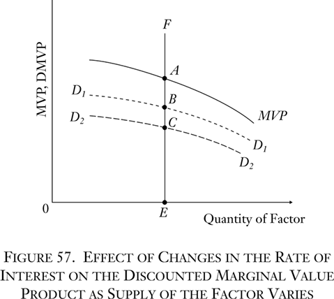
The supply of the factor is the EF line at the given quantity 0E. The solid line is the MVP schedule at various supplies. The MVP of the supply 0E is EA. Now the broken line D1D1 is the discounted marginal value product schedule at a certain rate of interest. Since it is discounted, it is uniformly lower than the MVP curve. In absolute terms, it is relatively lower at the left of the diagram, because an equal percentage drop implies a greater absolute drop where the amount is greater. The DMVP for supply 0E equals EB. EB will be the price of the factor in the evenly rotating economy.
Now suppose that the rate of interest in the economy rises, as a result, of course, of rises in time-preference schedules. This means that the rate of discount for every hypothetical MVP will be greater, and the absolute levels lower. The new DMVP schedule is depicted as the dotted line D2D2. The new price for the same supply of the factor is EC, a lower price than before.
One of the determinants of the DMVP schedule, then, is the rate of discount, and we have seen above that the rate of discount is determined by individual time preferences. The higher the rate of discount, the lower will tend to be the DMVP and, therefore, the lower the price of the factor; the lower the interest rate, the higher the DMVP and the price of the factor.
B. The Marginal Physical Product
B. The Marginal Physical Product
What, then, determines the position and shape of the MVP schedule? What is the marginal value product? It is the amount of revenue intake attributable to a unit of a factor. And this revenue depends on two elements: (1) the physical product produced and (2) the price of that product. If one hour of factor X is estimated by the market to produce a value of 20 gold ounces, this might be because one hour produces 20 units of the physical product, which are sold at a price of one gold ounce per unit. Or the same MVP might result from the production of 10 units of the product, sold at two gold ounces per unit, etc. In short, the marginal value product of a factor service unit is equal to its marginal physical product times the price of that product.6
Let us, then, investigate the determinants of the marginal physical product (MPP). In the first place, there can be no general schedule for the MPP as there is for the MVP, for the simple reason that physical units of various goods are not comparable. How can a dozen eggs, a pound of butter, and a house be compared in physical terms? Yet the same factor might be useful in the production of any of these goods. There can be an MPP schedule, therefore, only in particular terms, i.e., in terms of each particular production process in which the factor can be engaged. For each production process there will be for the factor a marginal physical production schedule of a certain shape. The MPP for a supply in that process is the amount of the physical product imputable to one unit of that factor, i.e., the amount of the product that will be lost if one unit of the factor is removed. If the supply of the factor in the process is increased by one unit, other factors remaining the same, then the MPP of the supply becomes the additional physical product that can be gained from the addition of the unit. The supply of the factor that is relevant for the MPP schedules is not the total supply in the society, but the supply in each process, since the MPP schedules are established for each process separately.
- 6This is not strictly true, but the technical error in the statement does not affect the causal analysis in the text. In fact, this argument is strengthened, for MVP actually equals MPP × “marginal revenue,” and marginal revenue is always less than, or equal to, price. See Appendix A below, “Marginal Physical and Marginal Value Product.”
(1) The Law of Returns
(1) The Law of Returns
In order to investigate the MPP schedule further, let us recall the law of returns, set forth in chapter 1. According to the law of returns, an eternal truth of human action, if the quantity of one factor varies, and the quantities of other factors remain constant, there is a point at which the physical product per factor is at a maximum. Physical product per factor may be termed the average physical product (APP). The law further states that with either a lesser or a greater supply of the factor the APP must be lower. We may diagram a typical APP curve as in Figure 58.

(2) Marginal Physical Product and Average Physical Product
(2) Marginal Physical Product and Average Physical Product
What is the relationship between the APP and MPP? The MPP is the amount of physical product that will be produced with the addition of one unit of a factor, other factors being given. The APP is the ratio of the total product to the total quantity of the variable factor, other factors being given. To illustrate the meanings of APP and MPP, let us consider a hypothetical case in which all units of other factors are constant, and the number of units of one factor is variable. In Table 13 the first column lists the number of units of the variable factor, and the second column the total physical product produced when these varying units are combined with fixed units of the other factors. The third column is the APP = total product divided by the number of units of the factor, i.e., the average physical productivity of a unit of the factor. The fourth column is the MPP = the difference in total product yielded by adding one more unit of the variable factor, i.e., the total product of the current row minus the total product of the preceding row:
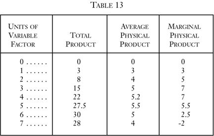
In the first place, it is quite clear that no factor will ever be employed in the region where the MPP is negative. In our example, this occurs where seven units of the factor are being employed. Six units of the factor, combined with given other factors, produced 30 units of the product. An addition of another unit results in a loss of two units of the product. The MPP of the factor when seven units are employed is -2. Obviously, no factor will ever be employed in this region, and this holds true whether the factor-owner is also owner of the product, or a capitalist hires the factor to work on the product. It would be senseless and contrary to the principles of human action to expend either effort or money on added factors only to have the quantity of the total product decline.
In the tabulation, we follow the law of returns, in that the APP, beginning, of course, at zero with zero units of the factor, rises to a peak and then falls. We also observe the following from our chart: (1) when the APP is rising (with the exception of the very first step where T P, APP, and MPP are all equal) MPP is higher than APP; (2) when the APP is falling, MPP is lower than APP; (3) at the point of maximum APP, MPP is equal to APP. We shall now prove, algebraically, that these three laws always hold.7
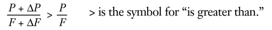
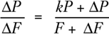
Let F be any number of units of a variable factor, other factors being given, and P be the units of the total product yielded by the combination. Then P/F is the Average Physical Product. When we add ΔF more units of the factor, total product increases by ΔP. Marginal Physical Product corresponding to the increase in the factor is ΔP/ΔF. The new Average Physical Product, corresponding to the greater supply of factors, is:

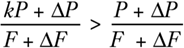
Now the new APP might be higher or lower than the previous one. Let us suppose that the new APP is higher and that therefore we are in a region where the APP is increasing. This means that:
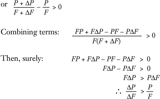
Thus, the MPP is greater than the old APP. Since it is greater, this means that there exists a positive number k such that:

Now there is an algebraic rule according to which, if:

then
Therefore,
Since k is positive,
Therefore,
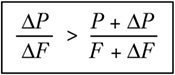
In short, the MPP is also greater than the new APP.
In other words, if APP is increasing, then the marginal physical product is greater than the average physical product in this region. This proves the first law above. Now, if we go back in our proof and substitute “less than” signs for “greater than” signs and carry out similar steps, we arrive at the opposite conclusion: where APP is decreasing, the marginal physical product is lower than the average physical product. This proves the second of our three laws about the relation between the marginal and the average physical product. But if MPP is greater than APP when the latter is rising, and is lower than APP when the latter is falling, then it follows that when APP is at its maximum, MPP must be neither lower nor higher than, but equal to, APP. And this proves the third law. We see that these characteristics of our table apply to all possible cases of production.
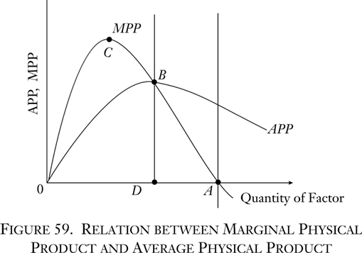
The diagram in Figure 59 depicts a typical set of MPP and APP schedules. It shows the various relationships between APP and MPP. Both curves begin from zero and are identical very close to their origin. The APP curve rises until it reaches a peak at B, then declines. The MPP curve rises faster, so that it is higher than APP, reaches its peak earlier at C, then declines until it intersects with APP at B. From then on, the MPP curve declines faster than APP, until finally it crosses the horizontal axis and becomes negative at some point A. No firm will operate beyond the 0A area.
Now let us explore further the area of increasing APP, between 0 and D. Let us take another hypothetical tabulation (Table 14), which will be simpler for our purpose.
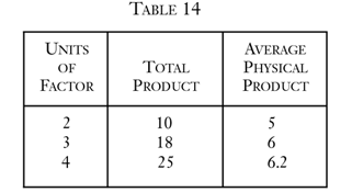
This is a segment of the increasing section of the average physical product schedule, with the peak being reached at four units and 6.2 APP. The question is: What is the likelihood that this region will be settled upon by a firm as the right input-output combination? Let us take the top line of the chart. Two units of the variable factor, plus a bundle of what we may call U units of all the other factors, yield 10 units of the product. On the other hand, at the maximum APP for the factor, four units of it, plus U units of other factors, yield 25 units of the product. We have seen above that it is a fundamental truth in nature that the same quantitative causes produce the same quantitative effects. Therefore, if we halve the quantities of all of the factors in the third line, we shall get half the product. In other words, two units of the factor combined with U/2—with half of the various units of each of the other factors—will yield 12.5 units of the product.
Consider this situation. From the top line we see that two units of the variable factor, plus U units of given factors, yield 10 units of the product. But, extrapolating from the bottom line, we see that two units of the variable factor, plus U/2 units of given factors, yield 12.5 units of the product. It is obvious that, as in the case of going beyond 0A, any firm that allocated factors so as to be in the 0D region would be making a most unwise decision. Obviously, no one would want to spend more in effort or money on factors (the “other” factors) and obtain less total output or, for that matter, the same total output. It is evident that if the producer remains in the 0D region, he is in an area of negative marginal physical productivity of the other factors. He would be in a situation where he would obtain a greater total product by throwing away some of the other factors. In the same way, after 0A, he would be in a position to gain greater total output if he threw away some of the present variable factor. A region of increasing APP for one factor, then, signifies a region of negative MPP for other factors, and vice versa. A producer, then, will never wish to allocate his factor in the 0D region or in the region beyond A.
Neither will the producer set the factor so that its MPP is at the points B or A. Indeed, the variable factor will be set so that it has zero marginal productivity (at A) only if it is a free good. There is however, no such thing as a free good; there is only a condition of human welfare not subject to action, and therefore not an element in productivity schedules. Conversely, the APP is at B, its maximum for the variable factor, only when the other factors are free goods and therefore have zero marginal productivity at this point. Only if all the other factors were free and could be left out of account could the producer simply concentrate on maximizing the productivity of one factor alone. However, there can be no production with only one factor, as we saw in chapter 1.
The conclusion, therefore, is inescapable. A factor will always be employed in a production process in such a way that it is in a region of declining APP and declining but positive MPP— between points D and A on the chart. In every production process, therefore, every factor will be employed in a region of diminishing MPP and diminishing APP so that additional units of the factor employed in the process will lower the MPP, and decreased units will raise it.
- 7It might be asked why we now employ mathematics after our strictures against the mathematical method in economics. The reason is that, in this particular problem, we are dealing with a purely technological question. We are not dealing with human decisions here, but with the necessary technological conditions of the world as given to human factors. In this external world, given quantities of cause yield given quantities of effect, and it is this sphere, very limited in the overall praxeological picture, that, like the natural sciences in general, is peculiarly susceptible to mathematical methods. The relationship between average and marginal is an obviously algebraic, rather than an ends-means, relation. Cf. the algebraic proof in Stigler, Theory of Price, pp. 44 ff.
C. Marginal Value Product
C. Marginal Value Product
As we have seen, the MVP for any factor is its MPP multiplied by the selling price of its product. We have just concluded that every factor will be employed in its region of diminishing marginal physical product in each process of production. What will be the shape of the marginal value product schedule? As the supply of a factor increases, and other factors remain the same, it follows that the total physical output of the product is greater. A greater stock, given the consumers’ demand curve, will lead to a lowering of the market price. The price of the product will then fall as the MPP diminishes and rise as the latter increases. It follows that the MVP curve of the factor will always be falling, and falling at a more rapid rate than the MPP curve. For each specific production process, any factor will be employed in the region of diminishing MVP.8 This correlates with the previous conclusion, based on the law of utility, that the factor in general, among various production processes, will be employed in such a way that its MVP is diminishing. Therefore, its general MVP (between various uses and within each use) is diminishing, and its various particular MVPs are diminishing (within each use). Its DMVP is, therefore, diminishing as well.
The price of a unit of any factor will, as we have seen, be established in the market as equal to its discounted marginal value product. This will be the DMVP as determined by the general schedule including all the various uses to which it can be put. Now the producers will employ the factor in such a way that its DMVP will be equalized among all the uses. If the DMVP in one use is greater than in another, then employers in the former line of production will be in a position to bid more for the factor and will use more of it until (according to the principle of diminishing MVP) the DMVP of the expanding use diminishes to the point at which it equals the increasing DMVP in the contracting use. The price of the factor will be set as equal to the general DMVP, which in the ERE will be uniform throughout all the particular uses.
Thus, by looking at a factor in all of its interrelations, we have been able to explain the pricing of its unit service without previously assuming the existence of the price itself. To focus the analysis on the situation as it looks from the vantage point of the firm is to succumb to such an error, for the individual firm obviously finds a certain factor price given on the market. The price of a factor unit will be established by the market as equal to its marginal value product, discounted by the rate of interest for the length of time until the product is produced, provided that this valuation of the share of the factor is isolable. It is isolable if the factor is nonspecific or is a single residual specific factor in a process. The MVP in question is determined by the general MVP schedule covering the various uses of the factor and the supply of the factor available in the economy. The general MVP schedule of a factor diminishes as the supply of the factor increases; it is made up of particular MVP schedules for the various uses of the factor, which in turn are compounded of diminishing Marginal Physical Product schedules and declining product prices. Therefore, if the supply of the factor increases, the MVP schedule in the economy remaining the same, the MVP and hence the price of the factor will drop; and as the supply of the factor dwindles, ceteris paribus, the price of the factor will rise.
To the individual firm, the price of a factor established on the market is the signal of its discounted marginal value product elsewhere. This is the opportunity cost of the firm’s using the product, since it equals the value product that is forgone through failure to use the factor unit elsewhere. In the ERE, where all factor prices equal discounted marginal value products, it follows that factor prices and (opportunity) “costs” will be equal.
Critics of the marginal productivity analysis have contended that in the “modern complex world” all factors co-operate in producing a product, and therefore it is impossible to establish any sort of imputation of part of the product to various co-operating factors. Hence, they assert, “distribution” of product to factors is separable from production and takes place arbitrarily according to bargaining theory. To be sure, no one denies that many factors do co-operate in producing goods. But the fact that most factors (and all labor factors) are nonspecific, and that there is very rarely more than one purely specific factor in a production process, enables the market to isolate value productivity and to tend to pay each factor in accordance with this marginal product. On the free market, therefore, the price of each factor is not determined by “arbitrary” bargaining, but tends to be set strictly in accordance with its discounted marginal value product. The importance of this market process becomes greater as the economy becomes more specialized and complex and the adjustments more delicate. The more uses develop for a factor, and the more types of factors arise, the more important is this market “imputation” process as compared to simple bargaining. For it is this process that causes the effective allocation of factors and the flow of production in accordance with the most urgent demands of the consumers (including the nonmonetary desires of the producers themselves). In the free-market process, therefore, there is no separation between production and “distribution.” There is no heap somewhere on which “products” are arbitrarily thrown and from which someone does or can arbitrarily “distribute” them among various people. On the contrary, individuals produce goods and sell them to consumers for money, which they in turn spend on consumption or on investment in order to increase future consumption. There is no separate “distribution”; there is only production and its corollary, exchange.
It should always be understood, even where it is not explicitly stated in the text for reasons of exposition, that the MVP schedules used to set prices are discounted MVP schedules, discounting the final MVP by the length of time remaining until the final consumers’ product is produced. It is the DMVPs that are equalized throughout the various uses of the factor. The importance of this fact is that it explains the market allocation of nonspecific factors among various productive stages of the same or of different goods. Thus, if the DMVP of a factor is six gold ounces, and if the factor is employed on a process practically instantaneous with consumption, its MVP will be six. Suppose that the pure rate of interest is 5 percent. If the factor is at work on a process that will mature in final consumption five years from now, a DMVP of six signifies an MVP of 7.5; if it is at work on a 10-year process, a DMVP of six signifies an MVP of 10; etc. The more remote the time of operation is from the time when the final product is completed, the greater must be the difference allowed for the annual interest income earned by the capitalists who advance present goods and thereby make possible the entire length of the production process. The amount of the discount from the MVP is greater here because the higher stage is more remote than the others from final consumption. Therefore, in order for investment to take place in the higher stages, their MVP has to be far higher than the MVP in the shorter processes.9