11. Money and Its Purchasing Power
11. Money and Its Purchasing Power
1. Introduction
1. Introduction
MONEY HAS ENTERED INTO ALMOST all our discussion so far. In chapter 3 we saw how the economy evolved from barter to indirect exchange. We saw the patterns of indirect exchange and the types of allocations of income and expenditure that are made in a monetary economy. In chapter 4 we discussed money prices and their formation, analyzed the marginal utility of money, and demonstrated how monetary theory can be subsumed under utility theory by means of the money regression theorem. In chapter 6 we saw how monetary calculation in markets is essential to a complex, developed economy, and we analyzed the structure of post-income and pre-income demands for and supplies of money on the time market. And from chapter 2 on, all our discussion has dealt with a monetary-exchange economy.
The time has come to draw the threads of our analysis of the market together by completing our study of money and of the effects of changes in monetary relations on the economic system. In this chapter we shall continue to conduct the analysis within the framework of the free-market economy.
2. The Money Relation: The Demand for and the Supply of Money
2. The Money Relation: The Demand for and the Supply of Money
Money is a commodity that serves as a general medium of exchange; its exchanges therefore permeate the economic system. Like all commodities, it has a market demand and a market supply, although its special situation lends it many unique features. We saw in chapter 4 that its “price” has no unique expression on the market. Other commodities are all expressible in terms of units of money and therefore have uniquely identifiable prices. The money commodity, however, can be expressed only by an array of all the other commodities, i.e., all the goods and services that money can buy on the market. This array has no uniquely expressible unit, and, as we shall see, changes in the array cannot be measured. Yet the concept of the “price” or the “value” of money, or the “purchasing power of the monetary unit,” is no less real and important for all that. It simply must be borne in mind that, as we saw in chapter 4, there is no single “price level” or measurable unit by which the value-array of money can be expressed. This exchange-value of money also takes on peculiar importance because, unlike other commodities, the prime purpose of the money commodity is to be exchanged, now or in the future, for directly consumable or productive commodities.
The total demand for money on the market consists of two parts: the exchange demand for money (by sellers of all other goods that wish to purchase money) and the reservation demand for money (the demand for money to hold by those who already hold it). Because money is a commodity that permeates the market and is continually being supplied and demanded by everyone, and because the proportion which the existing stock of money bears to new production is high, it will be convenient to analyze the supply of and the demand for money in terms of the total demand-stock analysis set forth in chapter 2.1
In contrast to other commodities, everyone on the market has both an exchange demand and a reservation demand for money. The exchange demand is his pre-income demand (see chapter 6, above). As a seller of labor, land, capital goods, or consumers’ goods, he must supply these goods and demand money in exchange to obtain a money income. Aside from speculative considerations, the seller of ready-made goods will tend, as we have seen, to have a perfectly inelastic (vertical) supply curve, since he has no reservation uses for the good. But the supply curve of a good for money is equivalent to a (partial) demand curve for money in terms of the good to be supplied. Therefore, the (exchange) demand curves for money in terms of land, capital goods, and consumers’ goods will tend to be perfectly inelastic.
For labor services, the situation is more complicated. Labor, as we have seen, does have a reserved use—satisfying leisure. We have seen that the general supply curve of a labor factor can be either “forward-sloping” or “backward-sloping,” depending upon the individuals’ marginal utility of money and marginal disutility of leisure forgone. In determining labor’s demand curve for money, however, we can be far more certain. To understand why, let us take a hypothetical example of a supply curve of a labor factor (in general use). At a wage rate of five gold grains an hour, 40 hours per week of labor service will be sold. Now suppose that the wage rate is raised to eight gold grains an hour. Some people might work a greater number of hours because they have a greater monetary inducement to sacrifice leisure for labor. They might work 50 hours per week. Others may decide that the increased income permits them to sacrifice some money and take some of the increased earnings in greater leisure. They might work 30 hours. The first would represent a “forward-sloping,” the latter a “backward-sloping,” supply curve of labor in this price range. But both would have one thing in common. Let us multiply hours by wage rate in each case, to arrive at the total money income of the laborers in the various situations. In the original case, a laborer earned 40 times 5 or 200 gold grains per week. The man with a backward-sloping supply curve will earn 30 times 8 or 240 gold grains a week. The one with a forward-sloping supply curve will earn 50 times 8 or 400 gold grains per week. In both cases, the man earns more money at the higher wage rate.
This will always be true. In the first case, it is obvious, for the higher wage rate induces the man to sell more labor. But it is true in the latter case as well. For the higher money income permits a man to gratify his desires for more leisure as well, precisely because he is getting an increased money income. Therefore, a man’s backward-sloping supply curve will never be “backward” enough to make him earn less money at higher wage rates.
Thus, a man will always earn more money at a higher wage rate, less money at a lower. But what is earning money but another name for buying money? And that is precisely what is done. People buy money by selling goods and services that they possess or can create. We are now attempting to arrive at the demand schedule for money in relation to various alternative purchasing powers or “exchange-values” of money. A lower exchange-value of money is equivalent to higher goods-prices in terms of money. Conversely, a higher exchange-value of money is equivalent to lower prices of goods. In the labor market, a higher exchange-value of money is translated into lower wage rates, and a lower exchange-value of money into higher wage rates.
Hence, on the labor market, our law may be translated into the following terms: The higher the exchange-value of money, the lower the quantity of money demanded; the lower the exchange-value of money, the higher the quantity of money demanded (i.e., the lower the wage rate, the less money earned; the higher the wage rate, the more money earned). Therefore, on the labor market, the demand-for-money schedule is not vertical, but falling, when the exchange-value of money increases, as in the case of any demand curve.
Adding the vertical demand curves for money in the other exchange markets to the falling demand curve in the labor market, we arrive at a falling exchange-demand curve for money.
More important, because more volatile, in the total demand for money on the market is the reservation demand to hold money. This is everyone’s post-income demand. After everyone has acquired his income, he must decide, as we have seen, between the allocation of his money assets in three directions: consumption spending, investment spending, and addition to his cash balance (“net hoarding”). Furthermore, he has the additional choice of subtraction from his cash balance (“net dishoarding”). How much he decides to retain in his cash balance is uniquely determined by the marginal utility of money in his cash balance on his value scale. Until now we have discussed at length the sources of the utilities and demands for consumers’ goods and for producers’ goods. We have now to look at the remaining good: money in the cash balance, its utility and demand.
Before discussing the sources of the demand for a cash balance, however, we may determine the shape of the reservation (or “cash balance”) demand curve for money. Let us suppose that a man’s marginal utilities are such that he wishes to have 10 ounces of money held in his cash balance over a certain period. Suppose now that the exchange-value of money, i.e., the purchasing power of a monetary unit, increases, other things being equal. This means that his 10 gold ounces accomplish more work than they did before the change in the PPM (purchasing power of the monetary unit). As a consequence, he will tend to remove part of the 10 ounces from his cash balance and spend it on goods, the prices of which have now fallen. Therefore, the higher the PPM (the exchange-value of money), the lower the quantity of money demanded in the cash balance. Conversely, a lower PPM will mean that the previous cash balance is worth less in real terms than it was before, while the higher prices of goods discourage their purchase. As a result, the lower the PPM, the higher the quantity of money demanded in the cash balance.
As a result, the reservation demand curve for money in the cash balance falls as the exchange-value of money increases. This falling demand curve, added to the falling exchange-demand curve for money, yields the market’s total demand curve for money—also falling in the familiar fashion for every commodity.
There is a third demand curve for the money commodity that deserves mention. This is the demand for nonmonetary uses of the monetary metal. This will be relatively unimportant in the advanced monetary economy, but it will exist nevertheless. In the case of gold, this will mean either uses in consumption, as for ornaments, or productive uses, as for industrial purposes. At any rate, this demand curve also falls as the PPM increases. As the “price” of money (PPM) increases, more goods can be obtained through expenditure of a unit of money; as a result, the opportunity-cost in using gold for nonmonetary purposes increases, and less is demanded for that purpose. Conversely, as the PPM falls, there is more incentive to use gold for its direct use. This demand curve is added to the total demand curve for money, to obtain the total demand curve for the money commodity.2
At any one time there is a given total stock of the money commodity. This stock will, at any time, be owned by someone. It is therefore dangerously misleading to adopt the custom of American economists since Irving Fisher’s day of treating money as somehow “circulating,” or worse still, as divided into “circulating money” and “idle money.”3 This concept conjures up the image of the former as moving somewhere at all times, while the latter sits idly in “hoards.” This is a grave error. There is, actually, no such thing as “circulation,” and there is no mysterious arena where money “moves.” At any one time all the money is owned by someone, i.e., rests in someone’s cash balance. Whatever the stock of money, therefore, people’s actions must bring it into accord with the total demand for money to hold, i.e., the total demand for money that we have just discussed. For even pre-income money acquired in exchange must be held at least momentarily in one’s cash balance before being transferred to someone else’s balance. All total demand is therefore to hold, and this is in accord with our analysis of total demand in chapter 2.
Total stock must therefore be brought into agreement, on the market, with the total quantity of money demanded. The diagram of this situation is shown in Figure 74.

On the vertical axis is the PPM, increasing upward. On the horizontal axis is the quantity of money, increasing rightwards. De is the aggregate exchange-demand curve for money, falling and inelastic.
Dr is the reservation or cash-balance demand for money. Dt is the total demand for money to hold (the demand for nonmonetary gold being omitted for purposes of convenience). Somewhere intersecting the Dt curve is the SS vertical line—the total stock of money in the community—given at quantity 0S.
The intersection of the latter two curves determines the equilibrium point, A, for the exchange-value of money in the community. The exchange-value, or PPM, will be set at 0B.
Suppose now that the PPM is slightly higher than 0B. The demand for money at that point will be less than the stock. People will become unwilling to hold money at that exchange-value and will be anxious to sell it for other goods. These sales will raise the prices of goods and lower the PPM, until the equilibrium point is reached. On the other hand, suppose that the PPM is lower than 0B. In that case, more people will demand money, in exchange or in reservation, than there is money stock available. The consequent excess of demand over supply will raise the PPM again to 0B.
- 1Cf. Edwin Cannan, “The Application of the Theoretical Analysis of Supply and Demand to Units of Currency” in F.A. Lutz and L.W. Mints, eds., Readings in Monetary Theory (Philadelphia: Blakiston, 1951), pp. 3–12, and Cannan, Money (6th ed.; London: Staples Press, 1929), pp. 10–19, 65–78.
- 2From this point on, this nonmonetary demand is included, for convenience, in the “total demand for money.”
- 3Cf. Irving Fisher, The Purchasing Power of Money (2nd ed.; New York: Macmillan & Co., 1913).
3. Changes in the Money Relation
3. Changes in the Money Relation
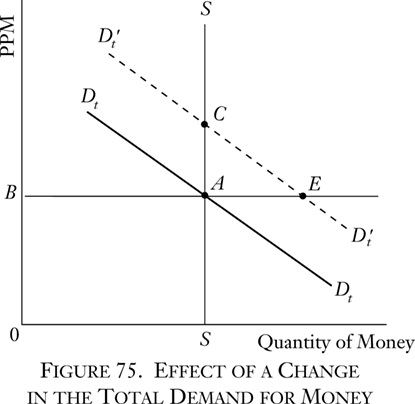
The purchasing power of money is therefore determined by two factors: the total demand schedule for money to hold and the stock of money in existence. It is easy to see on a diagram what happens when either of these determining elements changes. Thus, suppose that the schedule of total demand increases (shifts to the right). Then (see Figure 75) the total-demand-for-money curve has shifted from DtDt to Dt′Dt′. At the previous equilibrium PPM point, A, the demand for money now exceeds the stock available by AE. The bids push the PPM upwards until it reaches the equilibrium point C. The converse will be true for a shift of the total demand curve leftward—a decline in the total demand schedule. Then, the PPM will fall accordingly.
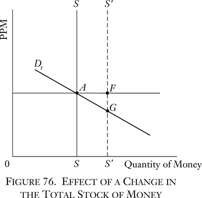
The effect of a change in the total stock, the demand curve remaining constant, is shown in Figure 76. Total quantity of stock increases from 0S to 0S′. At the new stock level there is an excess of stock, AF, over the total demand for money. Money will be sold at a lower PPM to induce people to hold it, and the PPM will fall until it reaches a new equilibrium point G. Conversely, if the stock of money is decreased, there will be an excess of demand for money at the existing PPM, and the PPM will rise until the new equilibrium point is reached.
The effect of the quantity of money on its exchange-value is thus simply set forth in our analysis and diagrams.
The absurdity of classifying monetary theories into mutually exclusive divisions (such as “supply and demand theory,” “quantity theory,” “cash balance theory,” “commodity theory,” “income and expenditure theory”) should now be evident.4 For all these elements are found in this analysis. Money is a commodity; its supply or quantity is important in determining its exchange-value; demand for money for the cash balance is also important for this purpose; and the analysis can be applied to income and expenditure situations.
- 4A typical such classification can be found in Lester V. Chandler, An Introduction to Monetary Theory (New York: Harper & Bros., 1940).
4. Utility of the Stock of Money
4. Utility of the Stock of Money
In the case of consumers’ goods, we do not go behind their subjective utilities on people’s value scales to investigate why they were preferred; economics must stop once the ranking has been made. In the case of money, however, we are confronted with a different problem. For the utility of money (setting aside the nonmonetary use of the money commodity) depends solely on its prospective use as the general medium of exchange. Hence the subjective utility of money is dependent on the objective exchange-value of money, and we must pursue our analysis of the demand for money further than would otherwise be required.5 The diagrams above in which we connected the demand for money and its PPM are therefore particularly appropriate. For other goods, demand in the market is a means of routing commodities into the hands of their consumers. For money, on the other hand, the “price” of money is precisely the variable on which the demand schedule depends and to which almost the whole of the demand for money is keyed. To put it in another way: without a price, or an objective exchange-value, any other good would be snapped up as a welcome free gift; but money, without a price, would not be used at all, since its entire use consists in its command of other goods on the market. The sole use of money is to be exchanged for goods, and if it had no price and therefore no exchange-value, it could not be exchanged and would no longer be used.
We are now on the threshold of a great economic law, a truth that can hardly be overemphasized, considering the harm its neglect has caused throughout history. An increase in the supply of a producers’ good increases, ceteris paribus, the supply of a consumers’ good. An increase in the supply of a consumers’ good (when there has been no decrease in the supply of another good) is demonstrably a clear social benefit; for someone’s “real income” has increased and no one’s has decreased.6
Money, on the contrary, is solely useful for exchange purposes. Money, per se, cannot be consumed and cannot be used directly as a producers’ good in the productive process. Money per se is therefore unproductive; it is dead stock and produces nothing. Land or capital is always in the form of some specific good, some specific productive instrument. Money always remains in someone’s cash balance.
Goods are useful and scarce, and any increment in goods is a social benefit. But money is useful not directly, but only in exchanges. And we have just seen that as the stock of money in society changes, the objective exchange-value of money changes inversely (though not necessarily proportionally) until the money relation is again in equilibrium. When there is less money, the exchange-value of the monetary unit rises; when there is more money, the exchange-value of the monetary unit falls. We conclude that there is no such thing as “too little” or “too much” money, that, whatever the social money stock, the benefits of money are always utilized to the maximum extent. An increase in the supply of money confers no social benefit whatever; it simply benefits some at the expense of others, as will be detailed further below. Similarly, a decrease in the money stock involves no social loss. For money is used only for its purchasing power in exchange, and an increase in the money stock simply dilutes the purchasing power of each monetary unit. Conversely, a fall in the money stock increases the purchasing power of each unit.
David Hume’s famous example provides a highly oversimplified view of the effect of changes in the stock of money, but in the present context it is a valid illustration of the absurdity of the belief that an increased money supply can confer a social benefit or relieve any economic scarcity. Consider the magical situation where every man awakens one morning to find that his monetary assets have doubled. Has the wealth, or the real income, of society doubled? Certainly not. In fact, the real income—the actual goods and services supplied—remains unchanged. What has changed is simply the monetary unit, which has been diluted, and the purchasing power of the monetary unit will fall enough (i.e., prices of goods will rise) to bring the new money relation into equilibrium.
One of the most important economic laws, therefore, is: Every supply of money is always utilized to its maximum extent, and hence no social utility can be conferred by increasing the supply of money.
Some writers have inferred from this law that any factors devoted to gold mining are being used unproductively, because an increased supply of money does not confer a social benefit. They deduce from this that the government should restrict the amount of gold mining. These critics fail to realize, however, that gold, the money-commodity, is used not only as money but also for nonmonetary purposes, either in consumption or in production. Hence, an increase in the supply of gold, although conferring no monetary benefit, does confer a social benefit by increasing the supply of gold for direct use.
5. The Demand for Money
5. The Demand for Money
A. Money in the ERE and in the Market
A. Money in the ERE and in the Market
It is true, as we have said, that the only use for money is in exchange. From this, however, it must not be inferred, as some writers have done, that this exchange must be immediate. Indeed, the reason that a reservation demand for money exists and cash balances are kept is that the individual is keeping his money in reserve for future exchanges. That is the function of a cash balance—to wait for a propitious time to make an exchange.
Suppose the ERE has been established. In such a world of certainty, there would be no risk of loss in investment and no need to keep cash balances on hand in case an emergency for consumer spending should arise. Everyone would therefore allocate his money stock fully, to the purchase of either present goods or future goods, in accordance with his time preferences. No one would keep his money idle in a cash balance. Knowing that he will want to spend a certain amount of money on consumption in six months’ time, a man will lend his money out for that period to be returned at precisely the time it is to be spent. But if no one is willing to keep a cash balance longer than instantaneously, there will be no money held and no use for a money stock. Money, in short, would either be useless or very nearly so in the world of certainty.
In the real world of uncertainty, as contrasted to the ERE, even “idle” money kept in a cash balance performs a use for its owner. Indeed, if it did not perform such a use, it would not be kept in his cash balance. Its uses are based precisely on the fact that the individual is not certain on what he will spend his money or of the precise time that he will spend it in the future.
Economists have attempted mechanically to reduce the demand for money to various sources.7 There is no such mechanical determination, however. Each individual decides for himself by his own standards his whole demand for cash balances, and we can only trace various influences which different catallactic events may have had on demand.
- 7J.M. Keynes’ Treatise on Money (New York: Harcourt, Brace, 1930) is a classic example of this type of analysis.
B. Speculative Demand
B. Speculative Demand
One of the most obvious influences on the demand for money is expectation of future changes in the exchange-value of money. Thus, suppose that, at a certain point in the future, the PPM of money is expected to drop rapidly. How the demand-for-money schedule now reacts depends on the number of people who hold this expectation and the strength with which they hold it. It also depends on the distance in the future at which the change is expected to take place. The further away in time any economic event, the more its impact will be discounted in the present by the interest rate. Whatever the degree of impact, however, an expected future fall in the PPM will tend to lower the PPM now. For an expected fall in the PPM means that present units of money are worth more than they will be in the future, in which case there will be a fall in the demand-for-money schedule as people tend to spend more money now than at the future date. A general expectation of an imminent fall in the PPM will lower the demand schedule for money now and thus tend to bring about the fall at the present moment.
Conversely, an expectation of a rise in the PPM in the near future will tend to raise the demand-for-money schedule as people decide to “hoard” (add money to their cash balance) in expectation of a future rise in the exchange-value of a unit of their money. The result will be a present rise in the PPM.
An expected fall in the PPM in the future will therefore lower the PPM now, and an expected rise will lead to a rise now. The speculative demand for money functions in the same manner as the speculative demand for any good. An anticipation of a future point speeds the adjustment of the economy toward that future point. Just as the speculative demand for a good speeded adjustment to an equilibrium position, so the anticipation of a change in the PPM speeds the market adjustment toward that position. Just as in the case of any good, furthermore, errors in this speculative anticipation are “self-correcting.” Many writers believe that in the case of money there is no such self-correction. They assert that while there may be a “real” or underlying demand for goods, money is not consumed and therefore has no such underlying demand. The PPM and the demand for money, they declare, can be explained only as a perpetual and rather meaningless cat-and-mouse race in which everyone is simply trying to anticipate everyone else’s anticipations.
There is, however, a “real” or underlying demand for money. Money may not be physically consumed, but it is used, and therefore it has utility in a cash balance. Such utility amounts to more than speculation on a rise in the PPM. This is demonstrated by the fact that people do hold cash even when they anticipate a fall in the PPM. Such holdings may be reduced, but they still exist, and as we have seen, this must be so in an uncertain world. In fact, without willingness to hold cash, there could be no monetary-exchange economy whatever.
The speculative demand therefore anticipates the underlying nonspeculative demands, whatever their source or inspiration. Suppose, then, that there is a general anticipation of a rise in the PPM (a fall in prices) not reflected in underlying supply and demand. It is true that, at first, this general anticipation raises, ceteris paribus, the demand for money and the PPM. But this situation does not last. For now that a pseudo “equilibrium” has been reached, the speculative anticipators, who did not “really” have an increased demand for money, sell their money (buy goods) to reap their gains. But this means that the underlying demand comes to the fore, and this is less than the money stock at that PPM. The pressure of spending then lowers the PPM again to the true equilibrium point. This may be diagramed as in Figure 77.

Money stock is 0S; the true or underlying money demand is DD, with true equilibrium point at A. Now suppose that the people on the market erroneously anticipate that true demand will be such in the near future that the PPM will be raised to 0E. The total demand curve for money then shifts to DsDs, the new total demand curve including the speculative demand. The PPM does shift to 0E as predicted. But now the speculators move to cash in their gain, since their true demand for money really reflects DD rather than DsDs. At the new price 0E, there is in fact an excess of money stock over quantity demanded, amounting to CF. Sellers rush to sell their stock of money and buy goods, and the PPM falls again to equilibrium. Hence, in the field of money as well as in that of specific goods, speculative anticipations are self-correcting, not “self-fulfilling.” They speed the market process of adjustment.
C. Secular Influences on the Demand for Money
C. Secular Influences on the Demand for Money
Long-run influences on the demand for money in a progressing economy will tend to be manifold, and in both directions. On the one hand, an advancing economy provides ever more occasions for new exchanges as more and more commodities are offered on the market and as the number of stages of production increases. These greater opportunities tend greatly to increase the demand-for-money schedule. If an economy deteriorates, fewer opportunities for exchange exist, and the demand for money from this source will fall.
The major long-run factor counteracting this tendency and tending toward a fall in the demand for money is the growth of the clearing system.8 Clearing is a device by which money is economized and performs the function of a medium of exchange without being physically present in the exchange.
A simplified form of clearing may occur between two people. For example, A may buy a watch from B for three gold ounces; at the same time, B buys a pair of shoes from A for one gold ounce. Instead of two transfers of money being made, and a total of four gold ounces changing hands, they decide to perform a clearing operation. A pays B two ounces of money, and they exchange the watch and the shoes. Thus, when a clearing is made, and only the net amount of money is actually transferred, all parties can engage in the same transactions at the same prices, but using far less cash. Their demand for cash tends to fall.
There is obviously little scope for clearing, however, as long as all transactions are cash transactions. For then people have to exchange one another’s goods at the same time. But the scope for clearing is vastly increased when credit transactions come into play. These credits may be quite short-term. Thus, suppose that A and B deal with each other quite frequently during a year or a month. Suppose they agree not to pay each other immediately in cash, but to give each other credit until the end of each month. Then B may buy shoes from A on one day, and A may buy a watch from B on another. At the end of the period, the debts are canceled and cleared, and the net debtor pays one lump sum to the net creditor.
Once credit enters the picture, the clearing system can be extended to as many individuals as find it convenient. The more people engage in clearing operations (often in places called “clearinghouses”) the more cancellations there will be, and the more money will be economized. At the end of the week, for example, there may be five people engaged in clearing, and A may owe B ten ounces, B owe C ten ounces, C owe D, etc., and finally E may owe A ten ounces. In such a case, 50 ounces’ worth of debt transactions and potential cash transactions are settled without a single ounce of cash being used.
Clearing, then, is a process of reciprocal cancellations of money debts. It permits a huge quantity of monetary exchanges without actual possession and transfer of money, thereby greatly reducing the demand for money. Clearing, however, cannot be all-encompassing, for there must be some physical money which could be used to settle the transaction, and there must be physical money to settle when there is no 100-percent cancellation (which rarely occurs).
- 8On the clearing system, see Mises, Theory of Money and Credit, pp. 281–86.
D. Demand for Money Unlimited?
D. Demand for Money Unlimited?
A popular fallacy rejects the concept of “demand for money” because it is allegedly always unlimited. This idea misconceives the very nature of demand and confuses money with wealth or income. It is based on the notion that “people want as much money as they can get.” In the first place, this is true for all goods. People would like to have far more goods than they can procure now. But demand on the market does not refer to all possible entries on people’s value scales; it refers to effective demand, to desires made effective by being “demanded,” i.e., by the fact that something else is “supplied” for it. Or else it is reservation demand, which takes the form of holding back the good from being sold. Clearly, effective demand for money is not and cannot be unlimited; it is limited by the appraised value of the goods a person can sell in exchange and by the amount of that money which the individual wants to spend on goods rather than keep in his cash balance.
Furthermore, it is, of course, not “money” per se that he wants and demands, but money for its purchasing power, or “real” money, money in some way expressed in terms of what it will purchase. (This purchasing power of money, as we shall see below, cannot be measured.) More money does him no good if its purchasing power for goods is correspondingly diluted.
E. The PPM and the Rate of Interest
E. The PPM and the Rate of Interest
We have been discussing money, and shall continue to do so in the current section, by comparing equilibrium positions, and not yet by tracing step by step how the change from one position to another comes about. We shall soon see that in the case of the price of money, as contrasted with all other prices, the very path toward equilibrium necessarily introduces changes that will change the equilibrium point. This will have important theoretical consequences. We may still talk, however, as if money is “neutral,” i.e., does not lead to such changes, because this assumption is perfectly competent to deal with the problems analyzed so far. This is true, in essence, because we are able to use a general concept of the “purchasing power of money” without trying to define it concretely in terms of specific arrays of goods. Since the concept of the PPM is relevant and important even though its specific content changes and cannot be measured, we are justified in assuming that money is neutral as long as we do not need a more precise concept of the PPM.
We have seen how changes in the money relation change the PPM. In the determination of the interest rate, we must now modify our earlier discussion in chapter 6 to take account of allocating one’s money stock by adding to or subtracting from one’s cash balance. A man may allocate his money to consumption, investment, or addition to his cash balance. His time preferences govern the proportion which an individual devotes to present and to future goods, i.e., to consumption and to investment. Now suppose a man’s demand-for-money schedule increases, and he therefore decides to allocate a proportion of his money income to increasing his cash balance. There is no reason to suppose that this increase affects the consumption/investment proportion at all. It could, but if so, it would mean a change in his time preference schedule as well as in his demand for money.
If the demand for money increases, there is no reason why a change in the demand for money should affect the interest rate one iota. There is no necessity at all for an increase in the demand for money to raise the interest rate, or a decline to lower it—no more than the opposite. In fact, there is no causal connection between the two; one is determined by the valuations for money, and the other by valuations for time preference.
Let us return to the section in chapter 6 on Time Preference and the Individual’s Money Stock. Did we not see there that an increase in an individual’s money stock lowers the effective time-preference rate along the time-preference schedule, and conversely that a decrease raises the time-preference rate? Why does this not apply here? Simply because we were dealing with each individual’s money stock and assuming that the “real” exchange-value of each unit of money remained the same. His time-preference schedule relates to “real” monetary units, not simply to money itself. If the social stock of money changes or if the demand for money changes, the objective exchange-value of a monetary unit (the PPM) will change also. If the PPM falls, then more money in the hands of an individual may not necessarily lower the time-preference rate on his schedule, for the more money may only just compensate him for the fall in the PPM, and his “real money stock” may therefore be the same as before. This again demonstrates that the money relation is neutral to time preference and the pure rate of interest.
An increased demand for money, then, tends to lower prices all around without changing time preference or the pure rate of interest Thus, suppose total social income is 100, with 70 allocated to investment and 30 to consumption. The demand for money increases, so that people decide to hoard a total of 20. Expenditure will now be 80 instead of 100, 20 being added to cash balances. Income in the next period will be only 80, since expenditures in one period result in the identical income to be allocated to the next period.9 If time preferences remain the same, then the proportion of investment to consumption in the society will remain roughly the same, i.e., 56 invested and 24 consumed. Prices and nominal money values and incomes fall all along the line, and we are left with the same capital structure, the same real income, the same interest rate, etc. The only things that have changed are nominal prices, which have fallen, and the proportion of total cash balances to money income, which has increased.
A decreased demand for money will have the reverse effect. Dishoarding will raise expenditure, raise prices, and, ceteris paribus, maintain the real income and capital structure intact. The only other change is a lower proportion of cash balances to money income.
The only necessary result, then, of a change in the demand-for-money schedule is precisely a change in the same direction of the proportion of total cash balances to total money income and in the real value of cash balances. Given the stock of money, an increased scramble for cash will simply lower money incomes until the desired increase in real cash balances has been attained.
If the demand for money falls, the reverse movement occurs. The desire to reduce cash balances causes an increase in money income. Total cash remains the same, but its proportion to incomes, as well as its real value, declines.10
- 9Since no one can receive a money income unless someone else makes a money expenditure on his services. (See chapter 3 above.)
- 10Strictly, the ceteris paribus condition will tend to be violated. An increased demand for money tends to lower money prices and will therefore lower money costs of gold mining. This will stimulate gold mining production until the interest return on mining is again the same as in other industries. Thus, the increased demand for money will also call forth new money to meet the demand. A decreased demand for money will raise money costs of gold mining and at least lower the rate of new production. It will not actually decrease the total money stock unless the new production rate falls below the wear-and-tear rate. Cf. Jacques Rueff, “The Fallacies of Lord Keynes’ General Theory” in Henry Hazlitt, ed., The Critics of Keynesian Economics (Princeton, N.J.: D. Van Nostrand, 1960), pp. 238–63.
F. Hoarding and the Keynesian System
F. Hoarding and the Keynesian System
(1) Social Income, Expenditures, and Unemployment
(1) Social Income, Expenditures, and Unemployment
To the great bulk of writers “hoarding”—an increase in the demand for money—has appeared an unmitigated catastrophe. The very word “hoarding” is a most inappropriate one to use in economics, since it is laden with connotations of vicious antisocial action. But there is nothing at all antisocial about either “hoarding” or “dishoarding.” “Hoarding” is simply an increase in the demand for money, and the result of this change in valuations is that people get what they desire, i.e., an increase in the real value of their cash balances and of the monetary unit.11 Conversely, if the people desire a lowering of their real cash balances or in the value of the monetary unit, they may accomplish this through “dishoarding.” No other significant economic relation—real income, capital structure, etc.—need be changed at all. The process of hoarding and dishoarding, then, simply means that people want something, either an increase or a decrease in their real cash balances or in the real value of the monetary unit, and that they are able to obtain this result. What is wrong with that? We see here simply another manifestation of consumers’ or individuals’ “sovereignty” on the free market.
Furthermore, there is no theoretical way of defining “hoarding” beyond a simple addition to one’s cash balance in a certain period of time. Yet most writers use the term in a normative fashion, implying that there is some vague standard below which a cash balance is legitimate and above which it is antisocial and vicious. But any quantitative limit set on the demand-for-money schedule would be completely arbitrary and unwarranted.
One of the two major pillars of the Keynesian system (now happily beginning to wane after sweeping the economic world in the 1930’s and 1940’s) is the proclamation that savings become equal to investment only through the terrible route of a decline in social income. The (implicit) foundation of Keynesianism is the assertion that at a certain level of total social income, total social expenditures out of this income will be lower than income, the remainder going into hoards. This will lower total social income in the next period of time, since, as we have seen, total income in one “day” equals, and is determined by, total expenditures in the previous “day.”
The Keynesian “consumption function” plays its part in establishing an alleged law that there exists a certain level of total income, say A, above which expenditures will be less than income (net hoarding), and below which expenditures will be greater than income (net dishoarding). But the basic Keynesian worry is hoarding, when total income must decline. This situation may be diagramed as in Figure 78.

In this graph, money income is plotted on both the horizontal and the vertical axes. Hence, a 45-degree straight line between the axes is equal to social income.12 To illustrate: A social income of 100 on the horizontal axis will correspond to, and equal, a social income of 100 on the vertical axis.
The coordinates of these figures will meet at a point equidistant between the two axes. The Keynesian law asserts social expenditures to be lower than social income above point A, and higher than social income below point A, so that A will be the equilibrium point for social income to equal expenditure. For if social income is higher than A, social expenditures will be lower than income, and income will therefore tend to decline from one day to the next until the equilibrium point A is reached. If social income is lower than A, dishoarding will occur, expenditures will be higher than income, until finally A is reached again.
Below, we shall investigate the validity of this alleged law and the “consumption function” on which it rests. But suppose that we now grant the validity of such a law; the only comment can be an impertinent: So what? What if there is a fall in the national income? Since the fall need only be in money terms, and real income, real capital, etc., may remain the same, why any alarm? The only change is that the hoarders have accomplished their objective of increasing their real cash balances and increasing the real value of the monetary unit. It is true that the picture is rather more complex for the transition process until equilibrium is reached, and this will be treated further below (although our final conclusion will be the same). But the Keynesian system attempts to establish the perniciousness of the equilibrium position, and this it cannot do.
Therefore, the elaborate attempts of the Keynesians to demonstrate that free-market expenditures will be limited—that consumption is limited by the “function,” and investment by stagnation of opportunities and “liquidity preference”—are futile. For even if they were correct (which they are not), the result would be pointless. There is nothing wrong with hoarding or dishoarding, or with “low” or “high” levels (whatever that may mean) of social money income.
The Keynesian attempt to salvage meaning for their doctrine rests on one point and one point alone—the second major pillar of their system. This is the thesis that money social income and level of employment are correlated, and that the latter is a function of the former. This assumes that a certain “full employment” level of social income exists below which there is correspondingly greater unemployment. This can be diagramed as in Figure 79.

On the previous diagram is superimposed a vertical FF line, which represents the point of alleged “full-employment” social income. If the intersection A is below (to the left of) the FF line, then there is permanent unemployment corresponding to the distance by which A falls short of that line.
Keynesians have also attempted, with little success, to give meaning to an equilibrium position where A falls to the right of the FF line, identifying this with inflation. Inflation, as we shall see below, is a dynamic process, the essence of which is change. The Keynesian system centers around the equilibrium position and therefore is hardly well equipped to analyze an inflationary situation.
The nub of the Keynesian critique of the free market economy, then, rests on the involuntary unemployment allegedly caused by too low a level of social expenditures and income. But how can this be, since we have previously explained that there can be no involuntary unemployment in a free market? The answer has become evident (and is admitted in the most intelligent of the Keynesian writings): The Keynesian “underemployment equilibrium” occurs only if money wage rates are rigid downward, i.e., if the supply curve of labor below “full employment” is infinitely elastic.13 Thus, suppose there is a “hoarding” (an increased demand for money), and social income falls. The result is a fall in the monetary demand curves for labor factors, as well as in all other monetary demand curves. We would expect the general supply curve of labor factors to be vertical. Since only money wage rates are being changed while real wage rates (in terms of purchasing power) remain the same, there will be no shift in labor/leisure preferences, and the total stock of labor offered on the market will remain constant. At any rate, certainly no involuntary unemployment will arise.
How then can the Keynesian case arise? How can the supply of labor remain horizontal at the old money wage rate? In only two ways: (1) if people voluntarily agree with the unions, which insist that no one be employed at lower than the old money wage rate. Since selling prices are falling, maintaining the old money wage rate is equivalent to demanding a higher real wage rate. We have seen above that the unions’ raising of real wage rates causes unemployment. But this unemployment is voluntary, since the workers acquiesce in the imposition of a higher minimum real wage rate, below which they will not undercut the union and accept employment. Or (2) unions or government coercively impose the minimum wage rate. But this is an example of a hampered market, not the free market to which we are confining our analysis here.
Situation (1) or (2) may be diagramed as in Figure 80.

The original demand curve for labor is DD (for simplicity of exposition we assume as meaningful the concept of “demand for labor” in general). Total stock of labor in the society is 0F, or at least that is the stock put forward upon the market. Now an increase in the demand for money shifts all demand curves downward as all money prices fall. If wage rates are free to fall, the intersection point will move from H to C and nominal wage rates reduced accordingly, from FH to FC.
There is still “full employment” at level 0F. Now suppose however, that a union sets a minimum money wage rate of 0B (or FH). Then the supply-of-labor curve becomes BHG; horizontal up to FG and vertical from there on. The new demand curve D′D′ will now intersect the supply of labor at point E instead of point C. Total amount of labor now employed is reduced to BE, and EH are now unemployed as a result of the union action.
Keynes’ own exposition tended to run in terms of real rather than money magnitudes—real social income, real expenditures, etc.14 Such an analysis obscures dynamic considerations, since transactions take place at least superficially in monetary terms on the market. However, the essential conclusion of our analysis remains unchanged if we pursue it directly in real terms. Instead of falling, demand curves in real terms will now remain the same. This is true for the labor market as well. Instead of being depicted on a diagram as a horizontal line at existing wage rates, the effect of union action would have to be shown as a horizontally imposed increase in real wage rates (the result of keeping money wage rates constant while selling prices fall). The relevant diagram is shown in Figure 81. The facts depicted in this diagram are the same as in the previous diagram: unions causing unemployment (EH) by insisting on an excessively high money (and therefore real) wage (0B).

The sum and substance of the “Keynesian Revolution” was the thesis that there can be an unemployment equilibrium on the free market. As we have seen, the only sense in which this is true was known years before Keynes: that widespread union maintenance of excessively high wage rates will cause unemployment.
Keynes believed that while other elements of the economic system, including prices, were set basically in real terms, workers bargained even ultimately only in terms of money wages—that unions insisted on minimum money wage rates downward, but would passively accept falling real wages in the form of rising prices, money wage rates remaining the same. The Keynesian prescription for eliminating unemployment therefore rests specifically on the “money illusion”—that unions will impose minimum money wage rates, but are too stupid to impose minimum real wage rates per se. Unions, however, have learned about purchasing-power problems and the distinction between money and real rates; indeed, it hardly requires much reasoning ability to grasp this distinction.15 Ironically, Keynes’ advocacy of inflation based on the “money illusion” rested on the historical experience (which we shall treat more fully below) that, during an inflation, selling prices rise faster than wage rates. Yet an economy in which unions impose minimum wage rates is precisely an economy in which unions will be alive to any losses in their real, as well as their money, wages. Inflation, therefore, cannot be used as a means of duping unions into relieving unemployment.16 Keynesianism has been touted as at least a “practical” system. Whatever its theoretical defects, it is alleged to be fit for the modern world of unionism. Yet it is precisely in the modern world that Keynes’ doctrine is least appropriate or practical.17
The Keynesians object that to allow rigid money wage rates to become flexible downward would further lower monetary demand for goods, and therefore monetary income. But this completely confuses wage rates with aggregate payroll, or total income going to wages.18 That the former falls does not mean that the latter falls. On the contrary, total income is, as we have seen, determined by total expenditures in the previous period of time. Lower wage rates will cause the hiring of those made unemployed by the old excessively high wage rates. The fact that labor is now cheaper relatively to land factors will cause investors to expend a greater proportion on labor visà-vis land than before. And the employment of unemployed labor increases production and therefore aggregate real income. Furthermore, even if payrolls also decline, prices and wage rates can adjust—but this will be taken up in the next section on liquidity preference.
- 11See the excellent article by W.H. Hutt, “The Significance of Price Flexibility” in Hazlitt, Critics of Keynseian Economics, pp. 383–406.
- 12The term generally used is “national” income. However, in a free-market economy the nation will no more be an important economic boundary than the village or region. It is more convenient, then, to set aside regional problems for other analysis and to concentrate on aggregate social income; this is especially true since regions do not present a problem to economic theory until their governments begin intervening in the free market.
- 13Thus, see the revealing article by Franco Modigliani, “Liquidity Preference and the Theory of Interest and Money” in Hazlitt, Critics of Keynesian Economics, pp. 156–69. Also see the articles by Erik Lindahl, “On Keynes’ Economic System—Part I,” The Economic Record, May, 1954, pp. 19–32; November, 1954, pp. 159–71; and Wassily W. Leontief, “Postulates: Keynes’ General Theory and the Classicists” in S. Harris, ed., The New Economics (New York: Knopf, 1952), pp. 232–42. For an empirical critique of the assumed Keynesian correspondence between aggregate output and employment, see George W. Wilson, “The Relationship between Output and Employment,” Review of Economics and Statistics, February, 1960, pp. 37–43.
- 14This is what Keynes’ discussion of “wage units” amounted to. Cf. Lindahl, “On Keynes’ Economic System—Part I,” p. 20.
- 15Cf. Lindahl, “On Keynes’ Economic System—Part I,” pp. 25, 159ff. Lindahl’s articles provide a good summary as well as a critique of the Keynesian system.
- 16Furthermore, inflation is, at best, an inefficient and distortive substitute for flexible wage rates. For inflation affects the entire economy and its prices, while particular wage rates will fall only to the extent necessary to “clear” the market for the particular labor factor. Thus, freely flexible wage rates will fall only in those fields necessary to eliminate unemployment in those particular areas. Cf. Henry Hazlitt, The Failure of the “New Economics” (Princeton, N.J.: D. Van Nostrand, 1959), pp. 278 ff.
- 17Cf. L. Albert Hahn, The Economics of Illusion (New York: Squier Publishing Co., 1949), pp. 50 ff., 166 ff., and passim.
(2) “Liquidity Preference”
(2) “Liquidity Preference”
Those Keynesians who recognize the grave difficulties of their system fall back on one last string in their bow—”liquidity preference.” Intelligent Keynesians will concede that involuntary unemployment is a “special” or rare case, and Lindahl goes even further to say that it could be only a short-run and not a long-run equilibrium phenomenon.19 Neither Modigliani nor Lindahl, however, is thoroughgoing enough in his critique of the Keynesian system, particularly of the “liquidity preference” doctrine.
The Keynesian system, as is quite clear from the mathematical portrayals of it given by its followers, suffers grievously from the mathematical-economic sin of “mutual determination.” The use of mathematical functions, which are reversible at will, is appropriate in physics, where we do not know the causes of the observed movements. Since we do not know the causes, any mathematical law explaining or describing movements will be reversible, and, as far as we are concerned, any of the variables in the function is just as much “cause” as another. In praxeology, the science of human action, however, we know the original cause—motivated action by individuals. This knowledge provides us with true axioms. From these axioms, true laws are deduced. They are deduced step by step in a logical, cause-and-effect relationship. Since first causes are known, their consequent effects are also known. Economics therefore traces unilinear cause-and-effect relations, not vague “mutually determining” relations.
This methodological reminder is singularly applicable to the Keynesian theory of interest. For the Keynesians consider the rate of interest (a) as determining investment and (b) as being determined by the demand for money to hold “for speculative purposes” (liquidity preference). In practice, however, they treat the latter not as determining the rate of interest, but as being determined by it. The methodology of “mutual determination” has completely obscured this sleight of hand. Keynesians might object that all demand and supply curves are “mutually determining” in their relation to price. But this facile assertion is not correct. Demand curves are determined by utility scales, and supply curves by speculation and the stock produced by given labor and land factors, which is ultimately governed by time preferences.
The Keynesians therefore treat the rate of interest, not as they believe they do—as determined by liquidity preference—but rather as some sort of mysterious and unexplained force imposing itself on the other elements of the economic system. Thus, Keynesian discussion of liquidity preference centers around “inducement to hold cash” as the rate of interest rises or falls. According to the theory of liquidity preference, a fall in the rate of interest increases the quantity of cash demanded for “speculative purposes” (liquidity preferences), and a rise in the rate of interest lowers liquidity preference.
The first error in this concept is the arbitrary separation of the demand for money into two separate parts: a “transactions demand,” supposedly determined by the size of social income, and a “speculative demand,” determined by the rate of interest. We have seen that all sorts of influences impinge themselves on the demand for money. But they are only influences working through the value scales of individuals. And there is only one final demand for money, because each individual has only one value scale. There is no way by which we can split the demand up into two parts and speak of them as independent entities. Furthermore, there are far more than two influences on demand. In the final analysis, the demand for money, like all utilities, cannot be reduced to simple determinants; it is the outcome of free, independent decisions on individual value scales. There is, therefore, no “transaction demand” uniquely determined by the size of income.
The “speculative demand” is mysterious indeed. Modigliani explains this “liquidity preference” as follows:
we should expect that any fall in the rate of interest ... would induce a growing number of potential investors to keep their assets in the form of money, rather than securities; that is to say, we should expect a fall in the rate of interest to increase the demand for money as an asset.20
This is subject to the criticism, as we have seen, that the rate of interest is here determining, and is not itself explained by any cause. Furthermore, what does this statement mean? A fall in the rate of interest, according to the Keynesians, means that less interest is being earned from bonds, and therefore there is a greater inducement to hold cash. This is correct (as long as we allow ourselves to think in terms of the interest rate as determining instead of being determined), but highly inadequate. For if a lower interest rate “induces” greater cash holdings, it also induces greater consumption, since consumption also becomes more attractive. In fact, one of the grave defects of the liquidity-preference approach is that the Keynesians never think in terms of three “margins” being decided at once. They think only in terms of two at a time. Hence, Modigliani: “Having made his consumption-saving plan, the individual has to make decisions concerning the assets he owns”; i.e., he then allocates them between money and securities.21 In other words, people first decide between consumption and saving (in the sense of not consuming); and then they decide between investing and hoarding these savings. But this is an absurdly artificial construction. People decide on all three of their alternatives, weighing one against each of the others. To say that people first decide between consuming and not consuming and then choose between hoarding and investing is just as misleading as to say that people first choose how much to hoard and then decide between consumption and investment.22
People, therefore, allocate their money among consumption, investment, and hoarding. The proportion between consumption and investment reflects individual time preferences. Consumption reflects desires for present goods, and investment reflects desires for future goods. An increase in the demand-for-money schedule does not affect the rate of interest if the proportion between consumption and investment (i.e., time preference) remains the same.
The rate of interest, we must reiterate, is determined by time preferences, which also determine the proportions of consumption and investment. To think of the rate of interest as “inducing” more or less saving or hoarding is to misunderstand the problem completely.23
Admitting, then, that time preference determines the proportions of consumption and investment and that the demand for money determines the proportion of income hoarded, does the demand for money play a role in determining the interest rate? The Keynesians assert that there is a relation between the rate of interest and a “speculative” demand for cash. Should the schedule of the latter rise, the former rises also. But this is not necessarily true. A greater proportion of funds hoarded can be drawn from three alternative sources: (a) from funds that formerly went into consumption, (b) from funds that went into investment, and (c) from a mixture of both that leaves the old consumption-investment proportion unchanged. Condition (a) will bring about a fall in the rate of interest; condition (b) a rise in the rate of interest, and condition (c) will leave the rate of interest unchanged. Thus hoarding may reflect either a rise, a fall, or no change in the rate of interest, depending on whether time preferences have concomitantly risen, fallen, or remained the same.
The Keynesians contend that the speculative demand for cash depends upon and determines the rate of interest in this way: if people expect that the rate of interest will rise in the near future, then their liquidity preference increases to await this rise. This, however, can hardly be a part of a long-run equilibrium theory, such as Keynes is trying to establish. Speculation, by its very nature, disappears in the ERE, and hence no fundamental causal theory can be based upon it. Furthermore, what is an interest rate? One grave and fundamental Keynesian error is to persist in regarding the interest rate as a contract rate on loans, instead of the price spreads between stages of production. The former, as we have seen, is only the reflection of the latter. A strong expectation of a rapid rise in interest rate means a strong expectation of an increase in the price spreads, or rate of net return. A fall in prices means that entrepreneurs generally expect that factor prices will fall further in the near future than their selling prices. But it requires no Keynesian labyrinth to explain this phenomenon; all we are confronted with is a situation in which entrepreneurs, expecting that factor prices will soon fall, cease investing and wait for this happy event so that their return will be greater. This is not “liquidity preference,” but speculation on price changes. It involves a modification of our previous discussion of the relation between prices and the demand for money, caused by a fact that we shall explore soon in detail, namely, that prices do not change equally and proportionately.
The expectation of falling factor prices speeds up the movement toward equilibrium and hence toward the pure interest relation as determined by time preference.24
If, for example, unions keep wage rates artificially high, “hoarding” will increase as unions keep wage rates ever higher than the equilibrium rate at which “full employment” can be maintained. This induced hoarding lowers the money demand for factors and increases unemployment still further, but only because of wage-rate rigidity.25
The final Keynesian bogey is that people may acquire an unlimited demand for money, so that hoards will indefinitely increase. This is termed an “infinite” liquidity preference. And this is the only case in which neo-Keynesians such as Modigliani believe that involuntary unemployment can be compatible with price and wage freedom. The Keynesian worry is that people will hoard instead of buying bonds for fear of a fall in the price of securities. Translating this into more important “natural” terms, this would mean, as we have stated, not investing because of expectation of imminent increases in the natural interest rate. Rather than act as a blockade, however, this expectation speeds the ensuing adjustment. Furthermore, the demand for money could not be infinite since people must always continue consuming, whatever their expectations. Of necessity, therefore, the demand for money could never be infinite. The existing level of consumption, in turn, will require a certain level of investment. As long as productive activities are continuing, there is no need or possibility of lasting unemployment, regardless of the degree of hoarding.26
A demand for money to hold stems from the general uncertainty of the market. Keynesians, however, attribute liquidity preference, not to general uncertainty, but to the specific uncertainty of future bond prices. Surely this is a highly superficial and limiting view.
In the first place, this cause of liquidity preference could occur only on a highly imperfect securities market. As Lachmann pointed out years ago in a neglected article, Keynes’ causal pattern—“bearishness” causing “liquidity preference” (demand for cash) and high interest rates—could take place only in the absence of an organized forward or futures market for securities.
If such a market existed, both bears and bulls on the bond market
could express their expectations by forward transactions which do not require any cash. Where the market for securities is fully organized over time, the owner of 4% bonds who fears a rise in the rate of interest has no incentive to exchange them for cash, for he can always “hedge” by selling them forward.27
Bearishness would cause a fall in forward bond prices, followed immediately by a fall in spot prices. Thus, speculative bearishness would, of course, cause at least a temporary rise in the rate of interest, but accompanied by no increase in the demand for cash. Hence, any attempted connection between liquidity preference, or demand for cash, and the rate of interest, falls to the ground.
The fact that such a securities market has not been organized indicates that traders are not nearly as worried about rising interest rates as Keynes believes. If they were and this fear loomed as an important phenomenon, then surely a futures market would have developed in securities.
Furthermore, as we have seen, interest rates on loans are merely a reflection of price spreads, so that a prediction of higher interest rates really means the expectation of lower prices and, especially, lower costs, resulting in a greater demand for money. And all speculation, on the free market, is self-correcting and speeds adjustment, rather than a cause of economic trouble.
- 19Cf. Lindahl’s critique of Lawrence Klein’s The Keynesian Revolution in “On Keynes’ Economic System—Part I,” p. 162. Also see Leontief, “Postulates: Keynes’ General Theory and the Classicists.”
- 20Modigliani, “Liquidity Preference and the Theory of Interest and Money,” pp. 139–40.
- 21Ibid., p. 137.
- 22See the critique of the Keynesian doctrine by Tjardus Greidanus, The Value of Money (2nd ed.; London: Staples Press, 1950), pp. 194–215, and of the liquidity-preference theory by D.H. Robertson, “Mr. Keynes and the Rate of Interest” in Readings in the Theory of Income Distribution, pp. 439–41. In contrast to Keynes’ famous phrase that the rate of interest is “the reward for parting with liquidity,” Greidanus points out that buying consumers’ goods (or even producers’ goods in Keynes’ sense of “interest”) sacrifices liquidity and yet earns no interest “reward.” Greidanus, Value of Money, p. 211. Also see Hazlitt, Failure of the “New Economics,” pp. 186 ff.
- 23Mises, Human Action, pp. 529–30.
- 24Hutt concludes that equilibrium
is secured when all services and products are so priced that they are (i) brought within the reach of people’s pockets (i.e., so that they are purchasable by existing money incomes) or (ii) brought into such a relation to predicted prices that no postponement of expenditure on them is induced. For instance, the products and services used in the manufacture of investment goods must be so priced that anticipated future money incomes will be able to buy the services and depreciation of new equipment or replacement. (Hutt, “Significance of Price Flexibility,” p. 394) - 25“Postponements (in purchases) arise because it is judged that a cut in costs (or other prices) is less than will eventually have to take place, or because the rate of fall of costs is insufficiently rapid.” Ibid., p. 395.
- 26As Hutt points out, if we can conceive of a situation of infinitely elastic liquidity preference (and no such situation has ever existed), then “we can conceive of prices falling rapidly, keeping pace with expectations of price changes, but never reaching zero, with full utilization of resources persisting all the way.” Ibid., p. 398.
- 27L.M. Lachmann, “Uncertainty and Liquidity Preference,” Economica, August, 1937, p. 301.
G. The Purchasing-Power and Terms-of-Trade Compenents in the Rate of Interest
G. The Purchasing-Power and Terms-of-Trade Compenents in the Rate of Interest
Many economists, beginning with Irving Fisher, have asserted that the market rate of interest, in addition to containing specific entrepreneurial components superimposed on the pure rate of interest, also contains a “price” or a “purchasing-power component.” When the purchasing power of money is generally expected to rise, the theory asserts that the market rate of interest falls correspondingly; when the PPM is expected to fall, the theory declares that the market rate of interest rises correspondingly.
These economists erred by concentrating on the loan rate rather than on the natural rate (the rate of return). The reasoning behind this theory was as follows: If the purchasing power of money is expected to change, then the pure rate of interest (determined by time preference) will no longer be the same in “real terms.” Suppose that 100 gold ounces exchange for 105 gold ounces a year from now—i.e., that the rate of interest is 5 percent. Now, suddenly, let there be a general expectation that the purchasing power of money will increase. In that case, a lower amount to be returned, say 102 ounces, may yield 5 percent real interest in terms of purchasing power. A general expectation of a rise in purchasing power, therefore, will lower the market rate of interest at present, while a general expectation of a fall in purchasing power will raise the rate.28
There is a fatal defect in this generally accepted line of reasoning. Suppose, for example, that prices are generally expected to fall by 50 percent in the next year. Would someone lend 100 gold ounces to exchange for 53 ounces one year from now? Why not? This would certainly preserve the real interest rate at 5 percent. But then why should the would-be lenders not simply hold on to their money and double their real assets as a result of the price fall? And that is precisely what they would do; they certainly would not give money away, even though their real assets would be greater than before. Fisher simply shrugged off this point by saying that the purchasing-power premium could never make the interest rate negative. But this flaw vitiates the entire theory.
The root of the difficulty consists in ignoring the natural rate of interest. Let us consider the interest rate in those terms. Then, suppose 100 ounces are paid for factors that will be transformed in one year into a product that sells for 105 gold ounces, for an interest gain of five and an interest return of 5 percent. Now a general expectation arises of a general halving of prices one year from now. The selling price of the product will be 53 ounces in a year’s time. What happens now? Will entrepreneurs buy factors for 100 and sell at 53 merely because their real interest rate is preserved? Certainly not. They will do so only if they do not at all anticipate the change in purchasing power. But to the extent that it is anticipated, they will hold money rather than buy factors. This will immediately lower factor prices to their expected future levels, say from 100 to 50.
What happens to the loan rate is analytically quite trivial. It is simply a reflection of the natural rate and depends on how the expectations and judgment of the people on the loan market compare with those on the stock and other markets. For the free economy, there is no point in separately analyzing the loan market. Analysis of the Fisher problem—the relation of the interest rate to price changes—should concentrate on the natural rate of interest. Discussion of the relation between price movements and the (natural) rate of interest should be divided into two parts: first, assuming “neutral money”—that all prices change equally and at the same time—and second, analyzing conditions where factor and product change at different rates. And these changes should first be analyzed without considering that they had been anticipated by people on the market.
Suppose, first, that all prices change equally and at the same time. Instead of thinking in terms of 100 ounces borrowed on the loan market, let us consider the natural rate. An investor buys factors in period 1 and then sells the product, say in period 3. Time, as we have seen, is the essence of the production structure. All the processes take time, and capitalists pay money to owners of factors in advance of production and sale. Since factors are bought before products are sold, what is the effect of a period of rising general prices (i.e., falling PPM)? The result is that the entrepreneur reaps an apparent extra profit. Suppose that he normally purchases original factors for 100 and then sells the product for 120 ounces two years later, for an interest return of 10 percent per annum. Now suppose that a decrease in the demand for money or an increase of money stock propels a general upward movement in prices and that all prices double in two years’ time. Then, just because of the passage of time, an entrepreneur who purchases factors for 100 now will sell for 240 ounces in two years’ time. Instead of a net return of 20 ounces, or 10 percent per annum, he reaps 140 ounces, or 70 percent per annum.
It would seem that a rise in prices creates an inherent tendency for large-scale profits that are not simply individual rewards for more accurate forecasting. However, more careful analysis reveals that this is not an extra profit at all. For the 240 ounces two years from now is roughly equivalent, in terms of purchasing power, to 120 ounces now. The real rate of net return, based on money’s services, is the same 10 percent as it has always been. It is clear that any lower net return would amount to a decline in real return. A return of a mere 120 ounces, for example, would amount to a drastic negative real return, for 100 ounces would then be invested for the equivalent gross return of only 60 ounces. It has often been shown that a period of rising prices misleads businessmen into thinking that their increased money profits are also real gains, whereas they only maintain real rates of return. Consider, for example, “replacement costs”—the prices which the businessmen will now have to pay for factors. The capitalist who earns 240 ounces on a 100-ounce investment neglects to his sorrow the fact that his factor bundle now costs 200 ounces instead of 100. Businessmen who under such circumstances treat their monetary profits as real profits and consume them soon find that they are really consuming their capital.
The converse occurs in the case of falling prices. The capitalist buys factors in period 1 and sells the product in period 3, when all-around prices are lower. If prices are to fall by a half in two years, an investment of 100, followed by a sale at 60, does not really involve the terrific loss that it appears to be. For the 60 return is equivalent in real terms, both in generalized purchasing power and in replacement of factors, to 120 previous ounces. His real rate of return remains the same. The consequence is that businessmen will be likely to overstate their losses in a period of price contraction. Perhaps this is one of the major reasons for the deep-seated belief of most businessmen that they always gain during a general price expansion and lose during a period of general contraction. This belief is purely illusory.
In these examples, the natural interest rate on the market has contained a purchasing-power component, which corrects for real rates, positively in money terms during a general expansion, and negatively during a general contraction. The loan rate will be simply a reflection of what has been happening in the natural rate. So far, the discussion is similar to Fisher’s, except that these are the effects of actual, not anticipated, changes and the Fisher thesis cannot take account of the negative interest rate case. We have seen that rather than take a monetary loss, even though their real return will be the same, entrepreneurs will hold back their purchases of factors until factor prices fall immediately to their future low level. But this process of anticipatory price movement does not occur only in the extreme case of a prospective “negative” return. It happens whenever a price change is anticipated. Thus, suppose all entrepreneurs generally anticipate that prices will double in two years. The fact of an anticipated rise will lead to an increase in the price level now and an approach immediately toward a doubled price level. An anticipated fall will lead to an immediate fall in factor prices. If all changes were anticipated by everyone, there would be no room for a purchasing-power component to develop. Prices would simply fall immediately to their future level.
The purchasing-power component, then, is not the reflection, as has been thought, of expectations of changes in purchasing power. It is the reflection of the change itself; indeed, if the change were completely anticipated, the purchasing power would change immediately, and there would be no room for a purchasing-power component in the rate of interest. As it is, partial anticipations speed up the adjustment of the PPM to the changed conditions.
So far we have distinguished three components of the natural rate of interest (all reflected in the loan rate of interest). One is the pure rate of interest—the result of individual time preferences, tending to be uniform throughout the economy. Second are the specific entrepreneurial rates of interest. These differ from firm to firm and so are not uniform. They are anticipated in advance, and they are the rates that an investor will have to anticipate receiving before he enters the field. A particularly “risky” venture, if successful at all, will therefore tend to earn more in net return than what is generally anticipated to be a “safe” venture. The third component of the natural rate of interest is the purchasing-power component, correcting for general PPM changes because of the inevitable time lags in production. This will be positive in an expansion and negative in a contraction, but will be ephemeral. The more that changes in the PPM are anticipated, the less important will be the purchasing-power component and the more rapid will be the adjustment in the PPM itself.
There is still a fourth component in the natural rate of interest. This exists to the extent that money changes are not neutral (and they never are). Sometimes product prices rise and fall faster than factor prices, sometimes they rise and fall more slowly, and sometimes their behavior is mixed, with some factor prices and some product prices rising more rapidly. Whenever there is a general divergence in rates of movement between the prices of the product and of original factors, a terms-of-trade component emerges in the natural rate of interest.
Historically, it has often been the case that product prices rise more rapidly and fall more rapidly than the prices of original factors. In the former case, there is, during the period of transition, a favorable change in the terms of trade to the general run of capitalists. For selling prices are increasing faster than the buying prices of original factors. This will increase the general rate of return and constitute a general positive terms-of-trade component in the natural rate of interest. This, of course, will also tend to be reflected in the loan rate of interest. In the case of a contraction, a more sluggish fall in the prices of factors creates a general negative terms-of-trade component in the interest rate. The components are precisely the reverse whenever factor prices change more rapidly than product prices. Whenever there is no general change in the “terms of trade” to capitalist-entrepreneurs, no terms-of-trade component will appear in the interest rate.
Changes in terms of trade discussed here are only those resulting purely from differences in the speed of reaction to changing conditions. They do not include basic changes in the terms of trade resulting from changes in time preferences, such as we have discussed above.
It is clear that all the interest-rate components aside from the pure rate—entrepreneurial, purchasing power, and terms of trade—are “dynamic” and the result of uncertainty. None of these components would exist in the ERE, and therefore the market interest rate in the ERE would equal the pure rate determined by time preferences alone. In the ERE the only net incomes would be a uniform pure interest return and wages to labor (ground land rents being capitalized into an interest return).
- 28Irving Fisher, The Rate of Interest (New York, 1907), chap. v, xiv; idem, Purchasing Power of Money, pp. 56–59.
6. The Supply of Money
6. The Supply of Money
A. The Stock of the Money Commodity
A. The Stock of the Money Commodity
The total stock of money in a society is the total number of ounces of the money commodity available. Throughout this volume we have deliberately used “gold ounces” instead of “dollars” or any other name for money, precisely because on the free market the latter would only be a confusing term for units of weight of gold or silver.
The total stock, from one period to another, will increase from new production and decrease from being used up—either in industrial production as a nonmonetary factor or from the wear and tear of coins. Since one of the qualities of the money commodity is its durability, the usual tendency is a long-run increase in the money supply and a resulting gradual long-run decline in the PPM. This furthers social utility only in so far as more gold or silver is made available for nonmonetary purposes.
We saw in chapter 3 that the physical form of the monetary commodity makes no difference. It can be in nonmonetary use as jewelry, in the form of bars of bullion, or in the form of coins. On the free market, transforming gold from one shape to another would be a business like any other business, charging a market price for its service and earning a pure interest return in the ERE. Since gold begins as bullion and ends as coin, it would seem that the latter would command a small premium over the equivalent weight of the former, the bullion often being a capital good for coin. Sometimes, however, coins are remelted back into bullion for larger transactions, so that a premium for coin over bullion is not a certainty. If, as generally happens, minting coins costs more than melting, coins will command the equivalent premium over bullion. This premium is called brassage.
It is impossible for economics to predict the details of the structure of any market. The market for privately issued gold bars or coins might develop as homogeneous, like the market for wheat, or the coins might be stamped and branded by the coin-makers to certify to the quality of their product. Probably the public would buy only branded coins to ensure accurate quality.
One argument against permitting free private coinage is that compulsory standardization of the denominations of coins is more convenient than the diversity of coins that would ensue under a free system. But if the market finds it more convenient, private mints will be led by consumer demand to mint certain standard denominations. On the other hand, if greater variety is preferred, consumers will demand and obtain a more varied number of coins.29
- 29For an exposition of the feasibility of private coinage, see Spencer, Social Statics, pp. 438–39; Charles A. Conant, The Principles of Money and Banking (New York: Harper & Bros., 1905), I, 127–32; Lysander Spooner, A Letter to Grover Cleveland (Boston: B.R. Tucker, 1886), p. 79; B.W. Barnard, “The Use of Private Tokens for Money in the United States,” The Quarterly Journal of Economics, 1916–17, pp. 617–26.
Recent writers favorable to private coinage include: Everett Ridley Taylor, Progress Report on a New Bill of Rights (Diablo, Calif.: the author, 1954); Oscar B. Johannsen, “Advocates Unrestricted Private Control over Money and Banking,” The Commercial and Financial Chronicle, June 12, 1958, pp. 2622f.; and Leonard E. Read, Government—An Ideal Concept (Irvington-on-Hudson, N.Y.: Foundation for Economic Education, 1954), pp. 82ff. An economist hostile to market-controlled commodity money has recently conceded the feasibility of private coinage under a commodity standard. Milton Friedman, A Program for Monetary Stability (New York: Fordham University Press, 1960), p. 5.
B. Claims to Money: The Money Warehouse
B. Claims to Money: The Money Warehouse
Chapter 2 described the difference between “claims to present goods” and “claims to future goods.” The same analysis applies to money as to barter. A claim to future money is a bill of exchange—an evidence of a credit transaction. The holder of the bill—the creditor—redeems it at the date of redemption in exchange for money paid by the debtor. A claim to present money, however, is a completely different good. It is not the evidence of an uncompleted transaction, an exchange of a present for a future good, as is the bill; it is a simple evidence of ownership of a present good. It is not uncompleted, or an exchange on the time market. Therefore, to present this evidence for redemption is not the completion of a transaction or equivalent to a creditor’s calling his loan; it is a simple repossessing of a man’s own good. In chapter 2 we gave as examples of a claim to present goods warehouse receipts and shares of stock. Shares of stock, however, cannot be redeemed in parts of a company’s fixed assets because of the rules of ownership that the companies themselves set up in their co-operative venture. Furthermore, there is no guarantee that such assets will have a fixed money value. We shall therefore confine ourselves to warehouse receipts, which are also more relevant to the supply of money.
When a man deposits goods at a warehouse, he is given a receipt and pays the owner of the warehouse a certain sum for the service of storage. He still retains ownership of the property; the owner of the warehouse is simply guarding it for him. When the warehouse receipt is presented, the owner is obligated to restore the good deposited. A warehouse specializing in money is known as a “bank.”
Claims to goods are often treated on the market as equivalent to the goods themselves. If no fraud or theft is suspected, then evidence of ownership of a good in a warehouse is considered as equivalent to the good itself. In many cases, individuals will find it advantageous to exchange the claims or evidences—the goods-substitutes—rather than the goods themselves. Paper is more convenient to transfer from person to person, and the expense of moving the goods is eliminated. When Jones sells Smith his wheat, therefore, instead of moving the wheat from one place to another, they may well agree simply to transfer the warehouse receipt itself from Jones to Smith. The goods remain in the same warehouse until Smith needs them or until the receipt is transferred to someone else. Of course, Smith may prefer, for one reason or another, to keep the goods in his own warehouse, in which case they are moved from one to the other.
Let us take the case of a warehouse owned by the Trustee Warehouse Company. It holds various goods in its vaults for safekeeping. Suppose that this company has developed a reputation for being very reliable and theft-free. Consequently, people tend to leave their goods in the Trustee Warehouse for a considerable length of time and, in the case of goods that they do not use frequently, will even tend to transfer the goods-certificates (the warehouse receipts, or evidences of ownership of the goods) and not redeem the goods themselves. Thus, the goods-certificates act as goods-substitutes in exchange. Suppose that the Trustee Company sees this happening. It realizes that a good opportunity for fraud presents itself. It can take the depositors’ goods, the goods that it holds for safekeeping, and lend them out to people on the market. It can earn interest on these loans, and as long as only a small percentage of depositors ask to redeem their certificates at any one time, no one is the wiser. Or, alternatively, it can issue pseudo warehouse receipts for goods that are not there and lend these on the market. This is the more subtle practice. The pseudo receipts will be exchanged on the market on the same basis as the true receipts, since there is no indication on their face whether they are legitimate or not.
It should be clear that this practice is outright fraud. Someone else’s property is taken by the warehouse and used for its own money-making purposes. It is not borrowed, since no interest is paid for the use of the money. Or, if spurious warehouse receipts are printed, evidences of goods are issued and sold or loaned without any such goods being in existence.
Money is the good most susceptible to these practices. For money, as we have seen, is generally not used directly at all, but only for exchanges. It is, furthermore, a widely homogeneous good, and therefore one ounce of gold is interchangeable with any other. Since it is convenient to transfer paper in exchange rather than carry gold, money warehouses (or banks) that build up public confidence will find that few people redeem their certificates. The banks will be particularly subject to the temptation to commit fraud and issue pseudo money certificates to circulate side by side with genuine money certificates as acceptable money-substitutes. The fact that money is a homogeneous good means that people do not care whether the money they redeem is the original money they deposited. This makes bank frauds easier to accomplish.
“Fraud” is a harsh term, but an accurate one to describe this practice, even if not recognized as such in the law, or by those committing it. It is, in fact, difficult to see the economic or moral difference between the issuance of pseudo receipts and the appropriation of someone else’s property or outright embezzlement or, more directly, counterfeiting. Most present legal systems do not outlaw this practice; in fact, it is considered basic banking procedure. Yet the libertarian law of the free market would have to prohibit it. The purely free market is, by definition, one where theft and fraud (implicit theft) are illegal and do not exist.
To part with goods or money held in trust or to issue spurious warehouse receipts is, of course, a dangerous business, even when the law permits it. If the warehouse once failed to meet its contractual obligations, its fraud would be discovered, and a general panic “run” on the warehouse or bank would ensue. It would then be quickly plunged into bankruptcy. Such a bankruptcy, however, would not be similar to the failure of an ordinary speculative business enterprise. It is rather similar to the absconder who gets caught before he has returned the funds he has “borrowed.”
Even if the receipt does not say on its face that the warehouse guarantees to keep it in its vaults, such an agreement is implicit in the very issuance of the receipt. For it is obvious that if any pseudo receipts are issued, it immediately becomes impossible for the bank to redeem all of them, and therefore fraud is immediately being committed. If a bank has 20 pounds of gold in its vaults, owned by depositors, and gold certificates redeemable on demand for 30 pounds, then notes to the value of 10 pounds are fraudulent. Which particular receipts are fraudulent can be determined only after a run on the bank has occurred and the later claimants are left unsatisfied.
In a purely free market where fraud cannot, by definition, occur, all bank receipts will be genuine, i.e., will represent only actual gold or silver in the vaults. In that case, all the bank’s money-substitutes (warehouse receipts) will also be money certificates, i.e., each receipt genuinely certifies the actual existence of the money in its vaults. The amount of gold kept in bank vaults for redemption purposes is called its “reserves,” and the policy of issuing only genuine receipts is therefore a policy of “100-percent reserves” of cash to demand liabilities (liabilities that must be paid on demand).30 However, the term “reserve” is a misleading one, because it assumes that the bank owns the gold and independently decides how much of it to keep on hand. Actually, it is not the bank that owns the gold, but its depositors.31
An enormous literature has developed dealing with the physical form of the money receipts, and yet the physical form is of no economic importance. It may be in the form of a paper note, a token coin (essentially a note stamped on coin instead of paper), or a book credit (demand deposit) in the bank. The demand deposit is not tangibly held by the owner, but can be transferred to anyone he desires by written order to the bank. This order is called a check. The depositor has a choice of which form of receipt to take, according to his convenience. Which form he chooses makes no economic difference.
- 30Time deposits are, legally, future claims, since banks have a legal right to delay payment 30 days. Moreover, they do not pass as final media of exchange. The latter fact is not determining, however, since a secure claim to a money-substitute is itself part of the money supply. “Idle” cash balances are kept as “time deposits,” just as gold bullion is a more “idle” form of money than coins. The deciding factor, perhaps, is that the 30-day limit is virtually a dead letter, for if a “savings” bank should impose it, a bankrupting “run” on the bank would ensue. Furthermore, actual payments are sometimes made by “cashiers’ checks” on time deposits. Thus, “time” deposits now function as demand deposits and should be treated as part of the money supply. If banks wished to act as genuine savings banks, borrowing and lending credit, they could issue I.O.U’s for specified lengths of time, due at definite future dates. Then no confusion or possible “counterfeiting” could arise.
- 31Such items as bills of lading, pawn tickets, and dock warrants have been warehouse receipts rooted in the specific objects deposited, in contrast to the loose “general deposits” where a homogeneous good can be returned. See W. Stanley Jevons, Money and the Mechanism of Exchange (16th ed.; London: Kegan Paul, Trench, Trübner & Co., 1907), pp. 201–11.
C. Money-Substitutes and the Supply of Money
C. Money-Substitutes and the Supply of Money
Since money-substitutes exchange as money on the market, we must consider them as part of the supply of money. It then becomes necessary to distinguish between money (in the broader sense)—the common medium of exchange—and money proper. Money proper is the ultimate medium of exchange or standard money—here the money commodity—while the supply of money (in a broader sense) includes all the standard money plus the money-substitutes that are held in individuals’ cash balances. In the cases cited above, gold was the money proper or standard money, while the receipts—the demand claims to gold—were the money-substitutes.
The relation between these elements may be illustrated as follows: Assume a community of three persons, A, B, C, and three money warehouses, X, Y, Z. Suppose that each person has 100 ounces of gold in his possession and none on deposit at a warehouse. For the community, then:

The total supply of money is here identical with the total supply of money proper.
Now assume that A and B each deposits his 100 ounces of gold at warehouses X and Y respectively, while C keeps his gold on hand. The total supply of money is always equal to the total of individual cash balances. Its composition now is:
A—100 ounces of X-Money-Substitute
B—100 ounces of Y-Money-Substitute
C—100 ounces of Gold Money Proper
Total supply of money (in the broader sense) = Total cash balances = 200 ounces of money-substitutes + 100 ounces of money proper.
The effect of the deposit of money proper in the warehouses or banks is to change the composition of the total supply of money in cash balances; the total amount, however, remains unchanged at 300 ounces. Money-substitutes of various banks have replaced most of the standard money in individual cash holdings. Similarly, if A and B were to redeem their deposits, the total amount would remain unchanged, while the composition would revert to the original pattern.
What of the 200 ounces of gold deposited in the vaults of the banks? These are no longer part of the money supply; they are held in reserve against the outstanding money-substitutes. While in reserve, they form no part of any individual’s cash balance; the cash balances consist not of the gold, but of evidences of ownership of the gold. Only the money proper outside of bank reserves forms part of individuals’ cash balances and hence part of the community’s supply of money.
Thus, as long as all money-substitutes are full money certificates, an increase or decrease in the money-substitutes outstanding can have no effect on the total supply of money. Only the composition of that supply is affected, and such changes in composition are of no economic importance.
However, when banks are legally permitted to abandon a 100-percent reserve and to issue pseudo receipts, the economic effects are quite different. We may call the money-substitutes that are not genuine money certificates, uncovered money-substitutes, since they do not genuinely represent money. The issue of uncovered money-substitutes adds to individuals’ cash balances and hence to the total supply of money. Uncovered money-substitutes are not offset by new money deposits and so constitute net additions to the total supply. Any increase or decrease in the supply of uncovered money-substitutes increases or decreases to the same extent the total supply of money (in the broader sense).
Thus, the total supply of money is composed of the following elements: supply of money proper outside reserves + supply of money certificates + supply of uncovered money-substitutes. The supply of money certificates has no effect on the size of the supply of money; an increase in this factor only decreases the size of the first factor. The supply of money proper and the factors determining its size have already been discussed. It depends on annual production compared to annual wear and tear, and thus, on the unhampered market, the supply of money-proper changes only slowly. As for uncovered money-substitutes, since they are essentially a phenomenon of the hampered rather than the free market, factors governing their supply will be further discussed below, in chapter 12.
In the meanwhile, however, let us analyze a little further the difference between a 100-percent-reserve and a fractional-reserve bank. The Star Bank, let us suppose, is a 100-percent-reserve bank; it is established with 100 gold ounces of capital invested by its stockholders in building and equipment. In the familiar balance sheet, with assets on the left-hand side and liabilities and capital on the right-hand side, the condition of the bank now appears as follows:

The Star Bank is ready to begin operations. Several people now come and deposit gold in the bank, which in return issues warehouse receipts giving the depositors (the true owners of the gold) the right to redeem their property on demand at any time. Let us assume that after a few months 5,000 gold ounces have been deposited and stored in the bank’s vaults. Its balance sheet now appears as follows:

The warehouse receipts function and exchange as money-substitutes, replacing, not adding to, the gold stored in the bank. All the warehouse receipts are money certificates, 100-percent reserve has been maintained, and no invasion of the free market has occurred. The warehouse receipts may take the form of printed tickets (notes) or book credit (demand deposits) transferable by written order or “check.” The two are economically identical.
But now suppose that law enforcement is lax and the bank sees that it can make money easily by engaging in fraud, i.e., by lending some of the depositors’ gold (or, rather, issuing pseudo warehouse receipts for nonexistent gold and lending them) to people who wish to borrow it.32 Let us say that the Star Bank, chafing at the mere interest return earned on its fees for warehouse service, prints 1,000 ounces of pseudo warehouse receipts and lends them on the credit market to businesses and consumers who desire to borrow money. The balance sheet of the Star Bank is now as follows:

The warehouse receipts still function as money-substitutes on the market. And we see that new money has been created by the bank out of thin air, as if by magic. This process of money creation has also been called the “monetization of debt,” an apt term since it describes the only instance where a liability can be transformed into money—the supreme asset. It is obvious that the more money the bank creates, the more profits it will earn, for any income earned on newly created money is a pure unalloyed gain. The bank has been able to alter the conditions of the free market system, in which money can be obtained only by purchase, mining, or gift. In each of these routes, productive service—either one’s own or one’s ancestor’s or benefactor’s—was necessary in order to obtain money. The bank’s inflationary intervention has created another route to money: the creation of new money out of thin air, by issuing receipts for nonexistent gold.33 ,34
- 32We might ask why the owners of the bank do not really reap the spoils and lend the money to themselves. The answer is that they once did so profusely, as the history of early American banking shows. Legal regulations forced the banks to abandon this practice.
- 33This discussion is not meant to imply that bankers, particularly at the present time, are always knowingly engaged in fraudulent practices. So embedded, indeed, have these practices become, and always with the sanction of law as well as of sophisticated but fallacious economic doctrines, that it is undoubtedly a rare banker who regards his standard occupational procedure as fraudulent.
- 34For a brilliant discussion of fractional-reserve banking, see Amasa Walker, The Science of Wealth (3rd ed.; Boston: Little, Brown & Co., 1867), pp. 138–68, 184–232.
D. A Note on Some Criticisms of 100-Percent Reserve
D. A Note on Some Criticisms of 100-Percent Reserve
One popular criticism of 100-percent bank reserves charges that the bank could not then earn any income or cover costs of storage, printing, etc. On the contrary, a bank is perfectly capable of operating like any goods warehouse, i.e., by charging its customers for its services to them and reaping the usual interest return on its operations.
Another popular objection is that a 100-percent-reserve policy would eliminate all credit. How would businessmen be able to borrow funds for short-term investment? The answer is that businessmen can still borrow saved funds from any individual or institution. “Banks” may still lend their own saved funds (capital stock and accumulated surplus) or they may borrow funds from individuals and relend them to business firms, earning the interest differential.35 Borrowing money (e g., floating a bond) is a credit transaction; an individual exchanges his present money for a bond—a claim on future money. The borrowing bank pays him interest for this loan and in turn exchanges the money thus gathered for promises by business borrowers to pay money in the future. This is a further credit transaction, in this case the bank acting as the lender and businesses as the borrowers. The bank’s income is the interest differential between the two types of credit transactions; the payment is for the services of the bank as an intermediary, channeling the savings of the public into investment. There is, furthermore, no particular reason why the short-term, more than any other, credit market should be subsidized by money creation.
Finally, an important criticism of a governmentally enforced policy of 100-percent reserves is that this measure, though beneficial in itself, would establish a precedent for other governmental intervention in the monetary system, including a change in this very requirement by government edict. These critics advocate “free banking,” i.e., no governmental interference with banking apart from enforcing payment of obligations, the banks to be permitted to engage in any fictitious issues they desire. Yet the free market does not mean freedom to commit fraud or any other form of theft. Quite the contrary. The criticism may be obviated by imposing a 100-percent-reserve requirement, not as an arbitrary administrative fiat of the government, but as part of the general legal defense of property against fraud. As Jevons stated: “It used to be held as a general rule of law, that any present grant or assignment of goods not in existence is without operation,”36 and this general rule need only be revived and enforced to outlaw fictitious money-substitutes. Then banking could be left perfectly free and yet be without departure from 100-percent reserves.37
- 35Swiss banks have successfully and for a long time been issuing debentures to the public at varying maturities, and banks in Belgium and Holland have recently followed suit. On the purely free market, such practices would undoubtedly be greatly extended. Cf. Benjamin H. Beck-hart, “ To Finance Term Loans,” The New York Times, May 31, 1960.
- 36Jevons, Money and the Mechanism of Exchange, pp. 211–12.
- 37Jevons stated:
If pecuniary promises were always of a special character, there could be no possible harm in allowing perfect freedom in the issue of promissory notes. The issuer would merely constitute himself a warehouse keeper and would be bound to hold each special lot of coin ready to pay each corresponding note. (Ibid., p. 208)
7. Gains and Losses During a Change in the Money Relation
7. Gains and Losses During a Change in the Money Relation
A change in the money relation necessarily involves gains and losses because money is not neutral and price changes do not take place simultaneously. Let us assume—and this will rarely hold in practice—that the final equilibrium position resulting from a change in the money relation is the same in all respects (including relative prices, individual values, etc.) as the previous equilibrium, except for the change in the purchasing power of money. Actually, as we shall see, there will almost undoubtedly be many changes in these factors in the new equilibrium situation. But even if there are not, the movement of prices from one equilibrium position to the next will not take place smoothly and simultaneously. It will not take place according to the famous example of David Hume and John Stuart Mill, where everyone awakens to find his money supply doubled overnight. Changes in the demand for money or the stock of money occur in step-by-step fashion, first having their effect in one area of the economy and then in the next. Because the market is a complex interacting network, and because some people react more quickly than others, movements of prices will differ in the speed of reaction to the changed situation.
As we have intimated above, the following law can be enunciated: When a change in the money relation causes prices to rise, the man whose selling price rises before his buying prices gains, and the man whose buying prices rise first, loses. The one who gains the most from the transition period is the one whose selling price rises first and buying prices last. Conversely, when prices fall, the man whose buying prices fall before his selling price gains, and the man whose selling price falls before his buying prices, loses.
It should be evident, in the first place, that there is nothing about rising prices that causes gains or about falling prices that causes losses. In either situation, some people gain and some people lose from the change, the gainers being the ones with the greatest and lengthiest positive differential between their selling and their buying prices, and the losers the ones with the greatest and longest negative differential in these movements. Which people gain and which lose from any given change is an empirical question, dependent on the location of changes in elements of the money relation, institutional conditions, anticipations, speeds of reaction, etc.
Let us consider the gains and losses from an increase in money stock. Suppose that we start from a position of monetary equilibrium. Every person’s money relation is in equilibrium, with his stock of and demand for money being equal. Now suppose that Mr. Jones finds some new gold never known before. A change in Jones’ data has taken place. He now has an excess stock of gold in his cash balance compared with his demand for it. Jones acts to spend his excess cash balance. This new money is spent, let us say, on the products of Smith. Smith now finds that his cash balance exceeds his demand for money, and he spends his excess on the products of someone else.
Jones’ increased supply also increases Smith’s selling price and income. Smith’s selling price has increased before his buying price. He spends the money on the products of Robinson, thus raising the latter’s selling prices while most buying prices have not risen. As the money is transferred from hand to hand, buying prices rise more and more. Robinson’s selling price increases, for example, but already one of the products he buys—Smith’s—has gone up. As the process continues, more and more buying prices rise. The individuals who are far down “on the list” to receive the new money, therefore, find that their buying prices have increased while their selling prices have not yet done so.
Of course, the changes in the money supply and in prices may well be insignificant. But this process occurs, however large or small the change in the money stock. Obviously, the larger the increase in money stock, the greater, ceteris paribus, will be its impact on prices.
We have seen above that an increase in the stock of money leads to a fall in the PPM, and a decrease in the stock of money leads to a rise in the PPM. However, there is no simple and uneventful rise and fall in the PPM. For a change in the stock of money is not automatically simultaneous. New money enters the system at some specific point and then becomes diffused in this way throughout the economy. The individuals who receive the new money first are the greatest gainers from the increased money; those who receive it last are the greatest losers, since all their buying prices have increased before their selling prices. Monetarily, it is clear that the gains of the approximate first half of the recipients of new money are exactly counterbalanced by the losses of the second half. Conversely, if money should somehow disappear from the system, say through wear and tear or through being misplaced, the initial loser cuts his spending and suffers most, while the last who feel the impact of a decreased money supply gain the most. For a decrease in the money supply results in losses for the first owners, who suffer a cut in selling price before their buying prices are lowered, and gains for the last, who see their buying prices fall before their income is cut.38
This analysis bears out our assertion above that there is no social utility in an increased supply, nor any social disutility in a decreased supply, of money. This is true for the transition period as well. An increase in gold is socially useful (i.e., beneficial to some without demonstrably injuring others) only to the extent that it makes possible an increase in the nonmonetary, direct use of gold.
If, as we have been assuming, relative prices and valuations remain the same for all throughout, the new equilibrium will be identical with the old except for an all-round price change. In that case, the gains and losses will be temporary, disappearing upon the advent of the new equilibrium. Actually, however, this will almost never occur. For even if people’s values remain frozen, the shift in relative money income during the transition itself changes the structure of demand. The gainers of wealth during the transition period will have a structure of preferences and demand different from that of the losers. As a result, demand itself will shift in structure, and the new equilibrium will have a different set of relative prices. Similarly, the change will probably not be neutral to time preferences. The permanent gainers will undoubtedly have a different structure of time preferences from that of the permanent losers, and, as a result, there may be a permanent shift in general time preferences. What the shift will be or in which direction, it is of course impossible for economics to say.
Money changes have this “driving force,” it may be noted, even in the fanciful case of the automatic overnight doubling of the supply of everyone’s cash balance. For the fact that everyone’s money stock doubles does not at all mean that all prices will automatically double! Each individual has a differently shaped demand-for-money schedule, and it is impossible to predict how each will be shaped. Some will spend proportionately more of their new money, and others will keep proportionately more in their cash balance. Many people will tend to spend their new cash balances on different goods from those they had bought with their old money. As a result, the structure of demand will change, and a decreased PPM will not double all prices; some will increase by more and some by less than double.39
8. The Determination of Prices: The Goods Side and the Money Side
8. The Determination of Prices: The Goods Side and the Money Side
We are now in a position to draw together all the strands determining the prices of goods. In chapters 4 through 9 we analyzed all the determinants of the prices of particular goods. In this chapter we have analyzed the determination of the purchasing power of money. Now we can see how both sets of determinants blend together.
A particular price, as we have seen, is determined by the total demand for the good (exchange and reservation) and the stock of the good, increasing as the former increases and decreasing as the latter increases. We may therefore call the demand a “factor of increase” of the price, and the stock a “factor of decrease.” The exchange demand for each good—the amount of money that will be spent in exchange for the good—equals the stock of money in the society minus the following: the exchange demands for all other goods and the reservation demand for money. In short, the amount spent on X good equals the total money supply minus the amount spent on other goods and the amount kept in cash balances.
Suppose we overlook the difficulties involved and now consider the price of “all goods,” i.e., the reciprocal of the purchasing power of money. The price of goods-in-general will now be determined by the monetary demand for all goods (factor of increase) and the stock of all goods (factor of decrease). Now, when all goods are considered, the exchange demand for goods equals the stock of money minus the reservation demand for money. (In contrast to any specific good, there is no need to subtract people’s expenditures on other goods.) The total demand for goods, then, equals the stock of money minus the reservation demand for money, plus the reservation demand for all goods.
The ultimate determinants of the price of all goods are: the stock of money and the reservation demand for goods (factors of increase), and the stock of all goods and the reservation demand for money (factors of decrease). Now let us consider the obverse side: the PPM. The PPM, as we have seen, is determined by the demand for money (factor of increase) and the stock of money (factor of decrease). The exchange demand for money equals the stock of all goods minus the reservation demand for all goods. Therefore, the ultimate determinants of the PPM are: the stock of all goods and the reservation demand for money (factors of increase), and the stock of money and the reservation demand for goods (factors of decrease). We see that this is the exact obverse of the determinants of the price of all goods, which, in turn, is the reciprocal of the PPM.
Thus, the analysis of the money side and the goods side of prices is completely harmonious. No longer is there need for an arbitrary division between a barter-type analysis of relative goods-prices and a holistic analysis of the PPM. Whether we treat one good or all goods, the price or prices will increase, ceteris paribus, if the stock of money increases; decrease when the stock of the good or goods increases; decrease when the reservation demand for money increases; and increase when the reservation demand for the good or goods increases. For each individual good, the price will also increase when the specific demand for that good increases; but unless this is a reflection of a drop in the social reservation demand for money, this changed demand will also signify a decreased demand for some other good, and a consequent fall in the price of the latter. Hence, changes in specific demands will not change the value of the PPM.
In a progressing economy, the secular trend for the four determining factors is likely to be: the money stock increasing gradually as gold production adds to the previous total; the stock of goods increasing as capital investment accumulates; the reservation demand for goods disappearing because short-run speculations disappear over the long run, and this is the main reason for such a demand; the reservation demand for money unknown, with clearing, for example, working to reduce this demand over a period of time, and the greater number of transactions tending to increase it. The result is that we cannot precisely say how the PPM will move in a progressing economy, though the best summary guess would be that it declines as a result of the influence of the increased stock of goods. Certainly, the influence of the goods side is in the direction of falling prices; the money side we cannot predict.
Thus, the ultimate determinants of the PPM as well as of specific prices are the subjective utilities of individuals (the determinants of demand) and the given objective stocks of goods—thereby vindicating the Austrian-Wicksteedian theory of price for all aspects of the economic system.
A final note of warning: It is necessary to remember that money can never be neutral. One set of conditions tending to raise the PPM can never precisely offset another set of factors tending to lower it. Thus, suppose that an increase in the stock of goods tends to raise the PPM, while at the same time, an increase in the money supply tends to lower it. One change can never offset the other; for one change will lower one set of prices more than others, while the other will raise a different set within the whole array of prices. The degrees of change in the two cases will depend on the particular goods and individuals affected and on their concrete valuations. Thus, even if we can make an historical (not an economic-scientific) judgment that the PPM has remained roughly the same, the price relations have shifted within the array, and therefore the judgment can never be exact.
9. Interlocal Exchange
9. Interlocal Exchange
A. Uniformity of the Geographic Purchasing Power of Money
A. Uniformity of the Geographic Purchasing Power of Money
The price of any commodity tends to be the same throughout the entire area using it. We have seen that this rule is not violated by the fact that cotton in Georgia, for example, is priced lower than cotton in New York. When cotton in New York is a consumers’ good, cotton in Georgia is a capital good in relation to the former. Cotton in Georgia is not the same commodity as cotton in New York because goods must first be processed in one location and then transported to the places where they are consumed.
Money is no exception to the rule that the price of every commodity will tend to be uniform throughout the entire area in which it is used. In fact, the scope for the money commodity is broader. Other commodities are produced in certain centers and must then be transported to other centers where they are consumed. They are therefore not the same “good” in different geographical locations; in the producing centers they are capital goods. Money, it is true, must first be mined and then shipped to places of use. But, once mined, the money commodity is used only for exchange. For these purposes, it is from then on shipped back and forth throughout the world market. Therefore, there is no really important capital-good location for money separate from a consumers’-good location. Whereas all other goods are first produced and then moved to the place where they are used and consumed, money is used interchangeably throughout the entire market area, moving back and forth. Therefore, the tendency toward geographical uniformity in the purchasing power of money holds true for the physical commodity gold or silver, and there is no need for that commodity to be treated as a different good in one place or another.
The purchasing power of money will therefore be identical over the entire area. Should the PPM be lower in New York than in Detroit, the supply of money for the exchange of goods will diminish in New York and increase in Detroit. Prices of goods being higher in New York than in Detroit, people will spend less in New York and more in Detroit than heretofore, this shift being reflected in the movement of money. This action will tend to raise the purchasing power of money in New York and lower it in Detroit, until its purchasing power in the two places is equal. The purchasing power of money will, in this way, tend to remain equal in all places where the money is used, whether or not national boundaries happen to intervene.
Some people contend that, on the contrary, there do exist permanent differences in the purchasing power of money from place to place. For example, they point to the fact that prices for food in restaurants are higher in New York City than in Peoria. For most people, however, New York has certain definite advantages over Peoria. It has a vastly wider range of goods and services available to the consumer, including theaters, concerts, colleges, high-quality jewelry and clothing, and stockbrokerage houses. There is a great difference between the commodity “restaurant service in New York” and the commodity “restaurant service in Peoria.” The former allows the purchaser to remain in New York and to enjoy its various advantages. Thus, the two are distinct goods, and the fact that the price of restaurant service is greater in New York signifies that the preponderance of individuals on the market value the former more highly and consider it a commodity of higher quality.40
Costs of transport, however, do introduce a qualification into this analysis. Suppose that the PPM in Detroit is slightly higher than in Rochester. We would expect gold to flow from Rochester to Detroit, spending relatively more on goods in the latter place, until the PPM’s are equalized. If, however, the PPM in Detroit is higher by an amount smaller than the transport cost of shipping the gold from Rochester, then relative PPM’s have a leeway to differ within the zone of shipping costs of gold. It would then be too expensive to ship gold to Detroit to take advantage of the higher PPM. The interspatial PPM’s may vary in either direction within this cost-of-transport margin.41
Many critics allege that the PPM cannot be uniform throughout the world because some goods are not transferable from one locale to another. Times Square or Niagara Falls, for example, cannot be transferred from one region to another; they are specific to their locale. Therefore, it is alleged, the equalization process can take place only for those goods which “enter into interregional trade”; it does not apply to the general PPM.
Plausible as it seems, this objection is completely fallacious. In the first place, disparate goods like Times Square and other main streets are different goods, so that there is no reason to expect them to have the same price. Secondly, so long as one commodity can be traded, the PPM can be equalized. The composition of the PPM may well be changed, but this does not refute the fact of equalization. The process of equalization can be deduced from the fact of human action, even though, as we shall see, the PPM cannot be measured, since its composition does not remain the same.
Finally, since any good can be traded, what is there to prevent, for example, Oshkosh capital from buying a building on Times Square? The Oshkosh capitalists need not literally transport a good back to Oshkosh in order to buy it and make money from their investment. Every good, then, “enters into interregional trade”; no distinction between “domestic” and “interregional” (or “international”) goods can be made.
Thus, suppose the PPM is higher in Oshkosh than in New York. New Yorkers tend to buy more in Oshkosh, and Oshkoshians will buy less in New York. This does not only mean that New York will buy more Oshkosh wheat, or that Oshkosh will buy less New York clothing. It also means that New Yorkers will invest in real estate or theaters in Oshkosh, while Oshkoshians will sell some of their New York holdings.
B. Clearing in Interlocal Exchange
B. Clearing in Interlocal Exchange
Clearing is particularly appropriate for interlocal transactions, since costs of transporting money from one locale to another are likely to be heavy. Bills of exchange on each town (i.e., I.O.U.’s owed by each town) can be reciprocally canceled. Suppose that there are two traders, A and B, in Detroit, and two in Rochester, C and D. A sells C a refrigerator for 200 gold grams, and D sells B a TV set for 200 grams. The two debts can be cleared, and no money need be shipped from one place to the other. On the other hand, D’s sale of a TV set may total 120 grams. Suppose for a moment that these are the only traders in the two communities. Then 80 grams will have to be shipped from Rochester to Detroit. In the latter case, the citizens of Detroit have, on net balance, decided to add to their cash holdings, while the Rochesterites have decided to diminish their cash holdings.
Economists have often described interlocal trade in terms of “gold export points” and “gold import points.” The use of such expressions assumes, however, that even though two localities both use gold money, it makes sense to talk of an “exchange rate” of the money of one locality for that of another. This exchange rate is set between the margins fixed by the cost of transporting money—the “gold import” and “gold export” points. This does not hold true on the free market, however. On such a market, all coins and bullion are expressed in terms of weight of gold, and it makes no sense whatever to speak of an “exchange rate” of the money of one place for the same money in another. How can there be an “exchange rate” of an ounce of gold for an ounce of gold? There will be no legal tender or other laws to separate the value of the coins of one area from those of another. Therefore, there may be slight variations in the PPM in each locale, within the limits of the cost of transporting gold, but there could never be deviations from par in interlocal “exchange rates.” For there are no exchange rates on the free market, except for two or more coexisting money commodities.
10. Balance of Payments
10. Balance of Payments
In chapter 3 above, we engaged in an extensive analysis of the individual’s balance of payments. We saw there that an individual’s income can be called his exports, and the physical sources of his income his goods exported; while his expenditures can be termed his imports, and the goods purchased his goods imported.42 We also saw that it is nonsensical to call a man’s balance of trade “favorable” if he chooses to use some of his income to add to his cash balance, or “unfavorable” if he decides to draw down his cash balance, so that expenditures are greater than income. Every action and exchange is favorable from the point of view of the person performing the action or exchange; otherwise he would not have engaged in it. A further conclusion is that there is no need for anyone to worry about anyone else’s balance of trade.
A person’s income and expenditure constitute his “balance of trade,” while his credit transactions, added to this balance, comprise his “balance of payment.” Credit transactions may complicate the balance, but they do not alter its essentials. When a creditor makes a loan, he adds to his “money paid” column to the extent of the loan—for purchase of a promise to pay in the future. He has purchased the debtor’s promise to pay in exchange for transferring part of his present cash balance to the debtor. The debtor adds to his “money receipts” column—from the sale of a promise to pay in the future. These promises to pay may fall due at any future date decided upon by the creditor and the debtor; generally they range from a day to many years. On that date the debtor repays the loan and transfers part of his cash balance to the creditor. This will appear in the debtor’s “money paid” column—for repayment of debt—and in the creditor’s “money received” column—from repayment of debt. Interest payments made by the debtor to the creditor will be similarly reflected in the respective balances of payments.
More nonsense has been written about balances of payments than about virtually any other aspect of economics. This has been caused by the failure of economists to ground and build their analysis on individual balances of payments. Instead they have employed such cloudy, holistic concepts as the “national” balance of payment without basing them on individual actions and balances.
Balances of payments may be consolidated for many individuals, and any number of groupings may be made. In these cases, the balances of payments only record the monetary transactions between individuals of the group and other individuals, but fail to record the exchanges of individuals within the group.
For example, suppose that we take the consolidated balance of payments for the Antlers Lodge of Jonesville for a certain period of time. There are three lodge members A, B, and C. Suppose their individual balances of payments are as indicated in Table 16.

In the consolidated balance sheet of the Antlers Lodge, the money payments between the members must of necessity cancel out. Thus,

The consolidated balance tells less about the activities of the members of the group than do the individual balances, since the exchanges within the group are not revealed. This discrepancy grows as the number of people grouped in the consolidated balance increases. The consolidated balance of the citizens of a large nation such as the United States conveys less information about their economic activities than is revealed by the consolidated balance of the citizens of Cuba. Finally, if we lump together all the citizens of the world engaged in exchange, their consolidated balance of payments is precisely zero. All the exchanges are internal within the group, and the consolidated balance conveys no information whatever about them. Taken together, the people of the world have zero income from “outside” and zero expenditures on “outside goods.”43
Fallacies in thinking about foreign trade will disappear if we understand that balances of payment are merely built upon consolidated individual transactions and that national balances are merely an arbitrary stopping point between individual balances on the one hand and the simple zeros of a world balance of payments on the other. There is, for example, the perennial worry that a balance of trade will be permanently “unfavorable” so that gold will drain out of the region in question until none is left. Drains of gold, however, are not mysterious acts of God. They are willed by people, who, on net balance, wish for one reason or another to reduce their cash balances of gold. The state of the balance is simply the visible manifestation of a voluntary reduction in the cash balance in a certain region or among a certain group.
Worries about national balances of payment are the fallacious residue of the accident that statistics of exchange are far more available across national boundaries than elsewhere. It should be clear that the principles applying to the balance of payment of the United States are the same for one region of the country, for one state, for one city, for one block, one house, or one person. Obviously no person or group can suffer because of an “unfavorable” balance; he or the group can suffer only because of a low level of income or assets. Seemingly plausible cries that money “be kept in” the United States, that Americans not be flooded with the “products of cheap foreign labor,” etc., take on a new perspective when we apply it, say, to a family of three Jones brothers. Imagine each brother exhorting the others to “buy Jones,” to “keep the money circulating within the Jones family,” to abstain from buying products made by others who earn less than the Jones family! Yet the principle of the argument is precisely the same in both cases.
Another popular argument is that a debtor group or nation cannot possibly repay its debt because its “balance of trade is in fundamental disequilibrium, being inherently unfavorable.” This is taken seriously in international affairs; yet how would we regard the individual debtor who used this excuse for defaulting on his loan? The creditor would be justified in bluntly telling the debtor that all he is saying is that he would much rather spend his money income and assets on enjoyable goods and services than on repayment of his debt. Except for the usual holistic analysis, we would see that the same holds true for an international debt.
11. Monetary Attributes of Goods
11. Monetary Attributes of Goods
Quasi Money
Quasi Money
We saw in chapter 3 how one or more very easily marketable commodities were chosen by the market as media of exchange, thereby greatly increasing their marketability and becoming more and more generally used until they could be called money. We have implicitly assumed that there are one or two media that are fully marketable—always salable—and other commodities that are simply sold for money. We have omitted mention of the degrees of marketability of these goods. Some goods are more readily marketable than others. And some are so easily marketable that they rise practically to the status of quasi moneys.
Quasi moneys do not form part of the nation’s money supply. The conclusive test is that they are not used to settle debts, nor are they claims to such means of payment at par. However, they are held as assets by individuals and are considered so readily marketable that an extra demand arises for them on the market. Their existence lowers the demand for money, since holders can economize on money by keeping them as assets. The price of these goods is higher than otherwise because of their quasi-monetary status.
In Oriental countries jewels have traditionally been held as quasi moneys. In advanced countries quasi moneys are usually short-term debts or securities that have a broad market and are readily salable at the highest price the market will yield. Quasi moneys include high-grade debentures, some stocks, and some wholesale commodities. Debentures used as quasi moneys have a higher price than otherwise and therefore a lower interest yield than will accrue on other investments.44
- 44Cf. Mises, Human Action, pp. 459–61.
B. Bills of Exchange
B. Bills of Exchange
In previous sections we saw that bills of exchange are not money-substitutes, but credit instruments. Money-substitutes are claims to present money, equivalent to warehouse receipts. But some critics maintain that in Europe at the turn of the nineteenth century bills did circulate as money-substitutes. They circulated as final payment in advance of their due dates, their face value discounted for the period of time left for maturity. Yet these were not money-substitutes. The holder of a bill was a creditor. Each of the acceptors of the bill had to endorse its payment, and the credit standing of each endorser had to be examined to judge the soundness of the bill. In short, as Mises has stated:
The endorsement of the bill is in fact not a final payment; it liberates the debtor to a limited degree only. If the bill is not paid then his liability is revived in a greater degree than before.45
Hence, the bills could not be classed as money-substitutes.
- 45Mises, Theory of Money and Credit, pp. 285–86.
12. Exchange Rates of Coexisting Moneys
12. Exchange Rates of Coexisting Moneys
Up to this point we have analyzed the market in terms of a single money and its purchasing power. This analysis is valid for each and every type of medium of exchange existing on the market. But if there is more than one medium coexisting on the market, what determines the exchange ratios between the various media? Although on an unhampered market there is a gradual tendency for one single money to be established, this tendency works very slowly. If two or more commodities offer good facilities and are both especially marketable, they may coexist as moneys. Each will be used by people as media of exchange.
For centuries, gold and silver were two commodities that coexisted as moneys. Both had similar advantages in scarcity, desirability for nonmonetary purposes, portability, durability, etc. Gold, however, being relatively far more valuable per unit of weight, was found to be more useful for larger transactions, and silver better for smaller transactions.
It is impossible to predict whether the market would have continued indefinitely to use gold and silver or whether one would have gradually ousted the other as a general medium of exchange. For, in the late nineteenth century, most Western countries conducted a coup d’etat against silver, to establish a monometallic standard by coercion.46 Gold and silver could and did coexist side by side in the same countries or throughout the world market, or one could function as money in one country, and one in another. Our analysis of the exchange rate is the same in both cases.
What determines the exchange rate between two (or more) moneys? Two different kinds of money will exchange in a ratio corresponding to the ratio of the purchasing power of each in terms of all the other economic goods. Thus, suppose that there are two coexisting moneys, gold and silver, and the purchasing power of gold is double that of silver, i.e., that the money price of every commodity is double in terms of silver what it is in terms of gold. One ounce of gold exchanges for 50 pounds of butter, and one ounce of silver exchanges for 25 pounds of butter. One ounce of gold will then tend to exchange for two ounces of silver; the exchange ratio of gold and silver will tend to be 1:2. If the rate at any time deviates from 1:2, market forces will tend to re-establish the parity between the purchasing powers and the exchange rate between them. This equilibrium exchange rate between two moneys is termed the purchasing power parity.
Thus, suppose that the exchange rate between gold and silver is 1:3, three ounces of silver exchanging for one ounce of gold. At the same time, the purchasing power of an ounce of gold is twice that of silver. It will now pay people to sell commodities for gold, exchange the gold for silver, and then exchange the silver back into commodities, thereby making a clear arbitrage gain. For example, people will sell 50 pounds of butter for one ounce of gold, exchange the gold for three ounces of silver, and then exchange the silver for 75 pounds of butter, gaining 25 pounds of butter. Similar gains from this arbitrage action will take place for all other commodities.
Arbitrage will restore the exchange rate between silver and gold to its purchasing power parity. The fact that holders of gold increase their demand for silver in order to profit by the arbitrage action will make silver more expensive in terms of gold and, conversely, gold cheaper in terms of silver. The exchange rate is driven in the direction of 1:2. Furthermore, holders of commodities are increasingly demanding gold to take advantage of the arbitrage, and this raises the purchasing power of gold. In addition, holders of silver are buying more commodities to make the arbitrage profit, and this action lowers the purchasing power of silver. Hence the ratio of the purchasing powers moves from 1:2 in the direction of 1:3. The process stops when the exchange rate is again at purchasing power parity, when arbitrage gains cease. Arbitrage gains tend to eliminate themselves and to bring about equilibrium.
It should be noted that, in the long run, the movement in the purchasing powers will probably not be important in the equilibrating process. With the arbitrage gains over, demands will probably revert back to what they were formerly, and the original ratio of purchasing powers will be restored. In the above case, the equilibrium rate will likely remain at 1:2.
Thus, the exchange rate between any two moneys will tend to be at the purchasing power parity. Any deviation from the parity will tend to eliminate itself and re-establish the parity rate. This holds true for any moneys, including those used mainly in different geographical areas. Whether the exchanges of moneys occur between citizens of the same or different geographical areas makes no economic difference, except for the costs of transport. Of course, if the two moneys are used in two completely isolated geographical areas with no exchanges between the inhabitants, then there is no exchange rate between them. Whenever exchanges do take place, however, the rate of exchange will always tend to be set at the purchasing power parity.
It is impossible for economics to state whether, if the money market had remained free, gold and silver would have continued to circulate side by side as moneys. There has been in monetary history a curious reluctance to allow moneys to circulate at freely fluctuating exchange ratios. Whether one of the moneys or both would be used as units of account would be up to the market to decide at its convenience.47
- 46For recent evidence that this action in the United States was a deliberate “crime against silver,” and not sheer accident, see Paul M. O’Leary, “The Scene of the Crime of 1873 Revisited,” Journal of Political Economy, August, 1960, pp. 388–92. One argument in favor of such action holds that the government thereby simplified accounts in the economy. However, the market could easily have done so itself by keeping all accounts in gold.
- 47See Mises, Theory of Money and Credit, pp. 179 ff., and Jevons, Money and the Mechanism of Exchange, pp. 88–96. For advocacy of such parallel standards, see Isaiah W. Sylvester, Bullion Certificates as Currency (New York, 1882); and William Brough, Open Mints and Free Banking (New York: G.P. Putnam’s Sons, 1894). Sylvester, who also advocated 100-percent specie-reserve currency, was an official of the United States Assay Office.
For historical accounts of the successful working of parallel standards, see Luigi Einaudi, “The Theory of Imaginary Money from Charlemagne to the French Revolution” in F.C. Lane and J.C. Riemersma, eds., Enterprise and Secular Change (Homewood, Ill.: Richard D. Irwin, 1953), pp. 229–61; Robert Sabatino Lopez, “Back to Gold, 1252,” Economic History Review, April, 1956, p. 224; and Arthur N. Young, “Saudi Arabian Currency and Finance,” The Middle East Journal, Summer, 1953, pp. 361–80.
13. The Fallacy of the Equation of Exchange
13. The Fallacy of the Equation of Exchange
The basis on which we have been explaining the purchasing power of money and the changes in and consequences of monetary phenomena has been an analysis of individual action. The behavior of aggregates, such as the aggregate demand for money and aggregate supply, has been constructed out of their individual components. In this way, monetary theory has been integrated into general economics. Monetary theory in American economics, however (apart from the Keynesian system, which we discuss elsewhere), has been presented in entirely different terms—in the quasi-mathematical, holistic equation of exchange, derived especially from Irving Fisher. The prevalence of this fallacious approach makes a detailed critique worthwhile.
The classic exposition of the equation of exchange was in Irving Fisher’s Purchasing Power of Money.48 Fisher describes the chief purpose of his work as that of investigating “the causes determining the purchasing power of money.” Money is a generally acceptable medium of exchange, and purchasing power is rightly defined as the “quantities of other goods which a given quantity of goods will buy.”49 He explains that the lower the prices of goods, the larger will be the quantities that can be bought by a given amount of money, and therefore the greater the purchasing power of money. Vice versa if the prices of goods rise. This is correct; but then comes this flagrant non sequitur: “In short, the purchasing power of money is the reciprocal of the level of prices; so that the study of the purchasing power of money is identical with the study of price levels.”50 From then on, Fisher proceeds to investigate the causes of the “price level”; thus, by a simple “in short,” Fisher has leaped from the real world of an array of individual prices for an innumerable list of concrete goods into the misleading fiction of a “price level,” without discussing the grave difficulties which any such concept must face. The fallacy of the “price level” concept will be treated further below.
The “price level” is allegedly determined by three aggregative factors: the quantity of money in circulation, its “velocity of circulation”—the average number of times during a period that a unit of money is exchanged for goods—and the total volume of goods bought for money. These are related by the famous equation of exchange: MV = PT. This equation of exchange is built up by Fisher in the following way: First, consider an individual exchange transaction—Smith buys 10 pounds of sugar for 7 cents a pound.51 An exchange has been made, Smith giving up 70 cents to Jones, and Jones transferring 10 pounds of sugar to Smith. From this fact Fisher somehow deduces that “10 pounds of sugar have been regarded as equal to 70 cents, and this fact may be expressed thus: 70 cents = 10 pounds multiplied by 7 cents a pound.”52 This off-hand assumption of equality is not self-evident, as Fisher apparently assumes, but a tangle of fallacy and irrelevance. Who has “regarded” the 10 pounds of sugar as equal to the 70 cents? Certainly not Smith, the buyer of the sugar. He bought the sugar precisely because he considered the two quantities as unequal in value; to him the value of the sugar was greater than the value of the 70 cents, and that is why he made the exchange. On the other hand, Jones, the seller of the sugar, made the exchange precisely because the values of the two goods were unequal in the opposite direction, i.e., he valued the 70 cents more than he did the sugar. There is thus never any equality of values on the part of the two participants. The assumption that an exchange presumes some sort of equality has been a delusion of economic theory since Aristotle, and it is surprising that Fisher, an exponent of the subjective theory of value in many respects, fell into the ancient trap. There is certainly no equality of values between two goods exchanged or, as in this case, between the money and the good. Is there an equality in anything else, and can Fisher’s doctrine be salvaged by finding such an equality? Obviously not; there is no equality in weight, length, or any other magnitude. But to Fisher, the equation represents an equality in value between the “money side” and the “goods side”; thus, Fisher states:
[T]he total money paid is equal in value to the total value of the goods bought. The equation thus has a money side and a goods side. The money side is the total money paid. ... The goods side is made up of the products of quantities of goods exchanged multiplied by respective prices.53
We have seen, however, that even for the individual exchange, and setting aside the holistic problem of “total exchanges,” there is no such “equality” that tells us anything about the facts of economic life. There is no “value-of-money side” equaling a “value-of-goods side.” The equal sign is illegitimate in Fisher’s equation.
How, then, account for the general acceptance of the equal sign and the equation? The answer is that, mathematically, the equation is of course an obvious truism: 70 cents = 10 pounds of sugar × 7 cents per pound of sugar. In other words, 70 cents = 70 cents. But this truism conveys no knowledge of economic fact whatsoever.54 Indeed, it is possible to discover an endless number of such equations, on which esoteric articles and books could be published. Thus:
Then, we could say that the “causal factors” determining the quantity of money are: the number of grains of sand, the number of students in the class, and the quantity of money. What we have in Fisher’s equation, in short, is two money sides, each identical with the other. In fact, it is an identity and not an equation. To say that such an equation is not very enlightening is self-evident. All that this equation tells us about economic life is that the total money received in a transaction is equal to the total money given up in a transaction—surely an uninteresting truism.
Let us reconsider the elements of the equation on the basis of the determinants of price, since that is our center of interest. Fisher’s equation of exchange for an individual transaction can be rearranged as follows:
Fisher considers that this equation yields the significant information that the price is determined by the total money spent divided by the total supply of goods sold. Actually, of course, the equation, as an equation, tells us nothing about the determinants of price; thus, we could set up an equally truistic equation:

This equation is just as mathematically true as the other, and, on Fisher’s own mathematical grounds, we could argue cogently that Fisher has “left the important wheat price out of the equation.” We could easily add innumerable equations with an infinite number of complex factors that “determine” price.
The only knowledge we can have of the determinants of price is the knowledge deduced logically from the axioms of praxeology. Mathematics can at best only translate our previous knowledge into relatively unintelligible form; or, usually, it will mislead the reader, as in the present case. The price in the sugar transaction may be made to equal any number of truistic equations; but it is determined by the supply and demand of the participants, and these in turn are governed by the utility of the two goods on the value scales of the participants in exchange. This is the fruitful approach in economic theory, not the sterile mathematical one. If we consider the equation of exchange as revealing the determinants of price, we find that Fisher must be implying that the determinants are the “70 cents” and the “10 pounds of sugar.” But it should be clear that things cannot determine prices. Things, whether pieces of money or pieces of sugar or pieces of anything else, can never act; they cannot set prices or supply and demand schedules. All this can be done only by human action: only individual actors can decide whether or not to buy; only their value scales determine prices. It is this profound mistake that lies at the root of the fallacies of the Fisher equation of exchange: human action is abstracted out of the picture, and things are assumed to be in control of economic life. Thus, either the equation of exchange is a trivial truism—in which case, it is no better than a million other such truistic equations, and has no place in science, which rests on simplicity and economy of methods—or else it is supposed to convey some important truths about economics and the determination of prices. In that case, it makes the profound error of substituting for correct logical analysis of causes based on human action, misleading assumptions based on action by things. At best, the Fisher equation is superfluous and trivial; at worst, it is wrong and misleading, although Fisher himself believed that it conveyed important causal truths.
Thus, Fisher’s equation of exchange is pernicious even for the individual transaction. How much more so when he extends it to the “economy as a whole”! For Fisher, this too was a simple step. “The equation of exchange is simply the sum of the equations involved in all individual exchanges”55 as in a period of time. Let us now, for the sake of argument, assume that there is nothing wrong with Fisher’s individual equations and consider his “summing up” to arrive at the total equation for the economy as a whole. Let us also abstract from the statistical difficulties involved in discovering the magnitudes for any given historical situation. Let us look at several individual transactions of the sort that Fisher tries to build into a total equation of exchange:
- exchanges 70 cents for 10 pounds of sugar
- exchanges 10 dollars for 1 hat
- exchanges 60 cents for 1 pound of butter
- exchanges 500 dollars for 1 television set.
What is the “equation of exchange” for this community of four? Obviously there is no problem in summing up the total amount of money spent: $511.30. But what about the other side of the equation? Of course, if we wish to be meaninglessly truistic, we could simply write $511.30 on the other side of the equation, without any laborious building up at all. But if we merely do this, there is no point to the whole procedure. Furthermore, as Fisher wants to get at the determination of prices, or “the price level,” he cannot rest content at this trivial stage. Yet he continues on the truistic level:
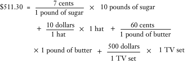
This is what Fisher does, and this is still the same trivial truism that “total money spent equals total money spent.” This triviality is not redeemed by referring to p × Q, p′ × Q′, etc., with each p referring to a price and each Q referring to the quantity of a good, so that: E = Total money spent = pQ + p′ Q′ + p″Q″ + ... etc. Writing the equation in this symbolic form does not add to its significance or usefulness.
Fisher, attempting to find the causes of the price level, has to proceed further. We have already seen that even for the individual transaction, the equation p = (E/Q) (price equals total money spent divided by the quantity of goods sold) is only a trivial truism and is erroneous when one tries to use it to analyze the determinants of price. (This is the equation for the price of sugar in Fisherine symbolic form.) How much worse is Fisher’s attempt to arrive at such an equation for the whole community and to use this to discover the determinants of a mythical “price level”! For simplicity’s sake, let us take only the two transactions of A and B, for the sugar and the hat. Total money spent, E, clearly equals $10.70, which, of course, equals total money received, pQ + p′Q′. But Fisher is looking for an equation to explain the price level; therefore he brings in the concept of an “average price level,” P, and a total quantity of goods sold, T, such that E is supposed to equal PT. But the transition from the trivial truism E = pQ + p′Q′ ... to the equation E = PT cannot be made as blithely as Fisher believes. Indeed, if we are interested in the explanation of economic life, it cannot be made at all.
For example, for the two transactions (or for the four), what is T? How can 10 pounds of sugar be added to one hat or to one pound of butter, to arrive at T? Obviously, no such addition can be performed, and therefore Fisher’s holistic T, the total physical quantity of all goods exchanged, is a meaningless concept and cannot be used in scientific analysis. If T is a meaningless concept, then P must be also, since the two presumably vary inversely if E remains constant. And what, indeed, of P? Here, we have a whole array of prices, 7 cents a pound, $10 a hat, etc. What is the price level? Clearly, there is no price level here; there are only individual prices of specific goods. But here, error is likely to persist. Cannot prices in some way be “averaged” to give us a working definition of a price level? This is Fisher’s solution. Prices of the various goods are in some way averaged to arrive at P, then P = (E/T), and all that remains is the difficult “statistical” task of arriving at T. However, the concept of an average for prices is a common fallacy. It is easy to demonstrate that prices can never be averaged for different commodities; we shall use a simple average for our example, but the same conclusion applies to any sort of “weighted average” such as is recommended by Fisher or by anyone else.
What is an average? Reflection will show that for several things to be averaged together, they must first be totaled. In order to be thus added together, the things must have some unit in common, and it must be this unit that is added. Only homogeneous units can be added together. Thus, if one object is 10 yards long, a second is 15 yards long, and a third 20 yards long, we may obtain an average length by adding together the number of yards and dividing by three, yielding an average length of 15 yards. Now, money prices are in terms of ratios of units: cents per pound of sugar, cents per hat, cents per pound of butter, etc. Suppose we take the first two prices:
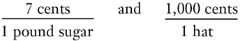
Can these two prices be averaged in any way? Can we add 1,000 and 7 together, get 1,007 cents, and divide by something to get a price level? Obviously not. Simple algebra demonstrates that the only way to add the ratios in terms of cents (certainly there is no other common unit available) is as follows:
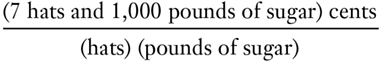
Obviously, neither the numerator nor the denominator makes sense; the units are incommensurable.
Fisher’s more complicated concept of a weighted average, with the prices weighted by the quantities of each good sold, solves the problem of units in the numerator but not in the denominator:
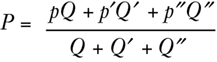
The pQ’s are all money, but the Q’s are still different units. Thus, any concept of average price level involves adding or multiplying quantities of completely different units of goods, such as butter, hats, sugar, etc., and is therefore meaningless and illegitimate. Even pounds of sugar and pounds of butter cannot be added together, because they are two different goods and their valuation is completely different. And if one is tempted to use poundage as the common unit of quantity, what is the pound weight of a concert or a medical or legal service?56
It is evident that PT, in the total equation of exchange, is a completely fallacious concept. While the equation E = pQ for an individual transaction is at least a trivial truism, although not very enlightening, the equation E = PT for the whole society is a false one. Neither P nor T can be defined meaningfully, and this would be necessary for this equation to have any validity. We are left only with E = pQ + p′Q′, etc., which gives us only the useless truism, E = E.57
Since the P concept is completely fallacious, it is obvious that Fisher’s use of the equation to reveal the determinants of prices is also fallacious. He states that if E doubles, and T remains the same, P—the price level—must double. On the holistic level, this is not even a truism; it is false, because neither P nor T can be meaningfully defined. All we can say is that when E doubles, E doubles. For the individual transaction, the equation is at least meaningful; if a man now spends $1.40 on 10 pounds of sugar, it is obvious that the price has doubled from 7 cents to 14 cents a pound. Still, this is only a mathematical truism, telling us nothing of the real causal forces at work. But Fisher never attempted to use this individual equation to explain the determinants of individual prices; he recognized that the logical analysis of supply and demand is far superior here. He used only the holistic equation, which he felt explained the determinants of the price level and was uniquely adapted to such an explanation. Yet the holistic equation is false, and the price level remains pure myth, an indefinable concept.
Let us consider the other side of the equation, E = MV, the average quantity of money in circulation in the period, multiplied by the average velocity of circulation. V is an absurd concept. Even Fisher, in the case of the other magnitudes, recognized the necessity of building up the total from individual exchanges. He was not successful in building up T out of the individual Q’s, P out of the individual p’s, etc., but at least he attempted to do so. But in the case of V, what is the velocity of an individual transaction? Velocity is not an independently defined variable. Fisher, in fact, can derive V only as being equal in every instance and every period to E/M. If I spend in a certain hour $10 for a hat, and I had an average cash balance (or M) for that hour of $200, then, by definition, my V equals 1/20. I had an average quantity of money in my cash balance of $200, each dollar turned over on the average of 1/20 of a time, and consequently I spent $10 in this period. But it is absurd to dignify any quantity with a place in an equation unless it can be defined independently of the other terms in the equation. Fisher compounds the absurdity by setting up M and V as independent determinants of E, which permits him to go to his desired conclusion that if M doubles, and V and T remain constant, P—the price level—will also double. But since V is defined as equal to E/M, what we actually have is: M × (E/M) = PT or simply, E = PT, our original equation. Thus, Fisher’s attempt to arrive at a quantity equation with the price level approximately proportionate to the quantity of money is proved vain by yet another route.
A group of Cambridge economists—Pigou, Robertson, etc.—has attempted to rehabilitate the Fisher equation by eliminating V and substituting the idea that the total supply of money equals the total demand for money. However, their equation is not a particular advance, since they keep the fallacious holistic concepts of P and T, and their k is merely the reciprocal of V, and suffers from the latter’s deficiencies.
In fact, since V is not an independently defined variable, M must be eliminated from the equation as well as V, and the Fisherine (and the Cambridge) equation cannot be used to demonstrate the “quantity theory of money.” And since M and V must disappear, there are an infinite number of other “equations of exchange” that we could, with equal invalidity, uphold as “determinants of the price level.” Thus, the aggregate stock of sugar in the economy may be termed S, and the ratio of E to the total stock of sugar may be called “average sugar turnover,” or U. This new “equation of exchange” would be: SU = PT, and the stock of sugar would suddenly become a major determinant of the price level. Or we could substitute A = number of salesmen in the country, and X = total expenditures per salesman, or “salesmen turnover,” to arrive at a new set of “determinants” in a new equation. And so on.
This example should reveal the fallacy of equations in economic theory. The Fisherine equation has been popular for many years because it has been thought to convey useful economic knowledge. It appears to be demonstrating the plausible (on other grounds) quantity theory of money. Actually, it has only been misleading.
There are other valid criticisms that could be made of Fisher: his use of index numbers, which even at best could only measure a change in a variable, but never define its actual position; his use of an index of T defined in terms of P and of P defined in terms of T; his denial that money is a commodity; the use of mathematical equations in a field where there can be no constants and therefore no quantitative predictions. In particular, even if the equation of exchange were valid in all other respects, it could at best only describe statically the conditions of an average period. It could never describe the path from one static condition to another. Even Fisher admitted this by conceding that a change in M would always affect V, so that the influence of M on P could not be isolated. He contended that after this “transition” period, V would revert to a constant and the effect on P would be proportional. Yet there is no reasoning to support this assertion. At any rate, enough has been shown to warrant expunging the equation of exchange from the economic literature.
- 48Fisher, Purchasing Power of Money, especially pp. 13 ff.
- 49Ibid., p. 13.
- 50Ibid., p. 14.
- 51We are using “dollars” and “cents” here instead of weights of gold for the sake of simplicity and because Fisher himself uses these expressions.
- 52Fisher, Purchasing Power of Money, p. 16.
- 53Ibid., p. 17.
- 54Greidanus justly calls this sort of equation “in all its absurdity the prototype of the equations set up by the equivalubrists,” in the modern mode of the “economics of the bookkeeper, not of the economist.” Greidanus, Value of Money, p. 196.
- 55Fisher, Purchasing Power of Money, p. 16.
- 56For a brilliant critique of the disturbing effects of averaging even when a commensurable unit does exist, see Louis M. Spadaro, “Averages and Aggregates in Economics” in On Freedom and Free Enterprise, pp. 140–60.
- 57See Clark Warburton, “Elementary Algebra and the Equation of Exchange,” American Economic Review, June, 1953, pp. 358–61. Also see Mises, Human Action, p. 396; B.M. Anderson, Jr., The Value of Money (New York: Macmillan & Co., 1926), pp. 154–64; and Greidanus, Value of Money, pp. 59–62.
14. The Fallacy of Measuring and Stabilizing the PPM
14. The Fallacy of Measuring and Stabilizing the PPM
A. Measurement
A. Measurement
In olden times, before the development of economic science, people naively assumed that the value of money remained always unchanged. “Value” was assumed to be an objective quantity inhering in things and their relations, and money was the measure, the fixed yardstick, of the values of goods and their changes. The value of the monetary unit, its purchasing power with respect to other goods, was assumed to be fixed.58 The analogy of a fixed standard of measurement, which had become familiar to the natural sciences (weight, length, etc.), was unthinkingly applied to human action.
Economists then discovered and made clear that money does not remain stable in value, that the PPM does not remain fixed. The PPM can and does vary, in response to changes in the supply of or the demand for money. These, in turn, can be resolved into the stock of goods and the total demand for money. Individual money prices, as we have seen in section 8 above, are determined by the stock of and demand for money as well as by the stock of and demand for each good. It is clear, then, that the money relation and the demand for and the stock of each individual good are intertwined in each particular price transaction. Thus, when Smith decides whether or not to purchase a hat for two gold ounces, he weighs the utility of the hat against the utility of the two ounces. Entering into every price, then, is the stock of the good, the stock of money, and the demand for money and the good (both ultimately based on individuals’ utilities). The money relation is contained in particular price demands and supplies and cannot, in practice, be separated from them. If, then, there is a change in the supply of or demand for money, the change will not be neutral, but will affect different specific demands for goods and different prices in varying proportions. There is no way of separately measuring changes in the PPM and changes in the specific prices of goods.
The fact that the use of money as a medium of exchange enables us to calculate relative exchange ratios between the different goods exchanged against money has misled some economists into believing that separate measurement of changes in the PPM is possible. Thus, we could say that one hat is “worth,” or can exchange for, 100 pounds of sugar, or that one TV set can exchange for 50 hats. It is a temptation, then, to forget that these exchange ratios are purely hypothetical and can be realized in practice only through monetary exchanges, and to consider them as constituting some barter-world of their own. In this mythical world, the exchange ratios between the various goods are somehow determined separately from the monetary transactions, and it then becomes more plausible to say that some sort of method can be found of isolating the value of money from these relative values and establishing the former as a constant yardstick. Actually, this barter-world is a pure figment; these relative ratios are only historical expressions of past transactions that can be effected only by and with money.
Let us now assume that the following is the array of prices in the PPM on day one:
- 10 cents per pound of sugar
- 10 dollars per hat
- 500 dollars per TV set
- 5 dollars per hour legal service of Mr. Jones, lawyer.
Now suppose the following array of prices of the same goods on day two:
- 15 cents per pound of sugar
- 20 dollars per hat
- 300 dollars per TV set
- 8 dollars per hour of Mr. Jones’ legal service.
Now what can economics say has happened to the PPM over these two periods? All that we can legitimately say is that now one dollar can buy 1/20 of a hat instead of 1/10 of a hat, 1/300 of a TV set instead of 1/500 of a set, etc. Thus, we can describe (if we know the figures) what happened to each individual price in the market array. But how much of the price rise of the hat was due to a rise in the demand for hats and how much to a fall in the demand for money? There is no way of answering such a question. We do not even know for certain whether the PPM has risen or declined. All we do know is that the purchasing power of money has fallen in terms of sugar, hats, and legal services, and risen in terms of TV sets. Even if all the prices in the array had risen we would not know by how much the PPM had fallen, and we would not know how much of the change was due to an increase in the demand for money and how much to changes in stocks. If the supply of money changed during this interval, we would not know how much of the change was due to the increased supply and how much to the other determinants.
Changes are taking place all the time in each of these determinants. In the real world of human action, there is no one determinant that can be used as a fixed benchmark; the whole situation is changing in response to changes in stocks of resources and products and to the changes in the valuations of all the individuals on the market. In fact, one lesson above all should be kept in mind when considering the claims of the various groups of mathematical economists: in human action there are no quantitative constants.59 As a necessary corollary, all praxeological-economic laws are qualitative, not quantitative.
The index-number method of measuring changes in the PPM attempts to conjure up some sort of totality of goods whose exchange ratios remain constant among themselves, so that a kind of general averaging will enable a separate measurement of changes in the PPM itself. We have seen, however, that such separation or measurement is impossible.
The only attempt to use index numbers that has any plausibility is the construction of fixed-quantity weights for a base period. Each price is weighted by the quantity of the good sold in the base period, these weighted quantities representing a typical “market basket” proportion of goods bought in that period. The difficulties in such a market-basket concept are insuperable, however. Aside from the considerations mentioned above, there is in the first place no average buyer or housewife. There are only individual buyers, and each buyer has bought a different proportion and type of goods. If one person purchases a TV set, and another goes to the movies, each activity is the result of differing value scales, and each has different effects on the various commodities. There is no “average person” who goes partly to the movies and buys part of a TV set. There is therefore no “average housewife” buying some given proportion of a totality of goods. Goods are not bought in their totality against money, but only by individuals in individual transactions, and therefore there can be no scientific method of combining them.
Secondly, even if there were meaning to the market-basket concept, the utilities of the goods in the basket, as well as the basket proportions themselves, are always changing, and this completely eliminates any possibility of a meaningful constant with which to measure price changes. The nonexistent typical housewife would have to have constant valuations as well, an impossibility in the real world of change.
All sorts of index numbers have been spawned in a vain attempt to surmount these difficulties: quantity weights have been chosen that vary for each year covered; arithmetical, geometrical, and harmonic averages have been taken at variable and fixed weights; “ideal” formulas have been explored—all with no realization of the futility of these endeavors. No such index number, no attempt to separate and measure prices and quantities, can be valid.60
- 58Conventional accounting practice is based on a fixed value of the monetary unit.
- 59Professor Mises has pointed out that the assertion of the mathematical economists that their task is made difficult by the existence of “many variables” in human action grossly understates the problem; for the point is that all the determinants are variables and that in contrast to the natural sciences there are no constants.
- 60See the brilliant critique of index numbers by Mises, Theory of Money and Credit, pp. 187–94. Also see R.S. Padan, “Review of C.M. Walsh’s Measurement of General Exchange Value,” Journal of Political Economy, September, 1901, p. 609.
B. Stabilization
B. Stabilization
The knowledge that the purchasing power of money could vary led some economists to try to improve on the free market by creating, in some way, a monetary unit which would remain stable and constant in its purchasing power. All these stabilization plans, of course, involve in one way or another an attack on the gold or other commodity standard, since the value of gold fluctuates as a result of the continual changes in the supply of and the demand for gold. The stabilizers want the government to keep an arbitrary index of prices constant by pumping money into the economy when the index falls and taking money out when it rises. The outstanding proponent of “stable money,” Irving Fisher, revealed the reason for his urge toward stabilization in the following autobiographical passage: “I became increasingly aware of the imperative need of a stable yardstick of value. I had come into economics from mathematical physics, in which fixed units of measure contribute the essential starting point.”61 Apparently, Fisher did not realize that there could be fundamental differences in the nature of the sciences of physics and of purposeful human action.
It is difficult, indeed, to understand what the advantages of a stable value of money are supposed to be. One of the most frequently cited advantages, for example, is that debtors will no longer be harmed by unforeseen rises in the value of money, while creditors will no longer be harmed by unforeseen declines in its value. Yet if creditors and debtors want such a hedge against future changes, they have an easy way out on the free market. When they make their contracts, they can agree that repayment be made in a sum of money corrected by some agreed-upon index number of changes in the value of money. Such a voluntary tabular standard for business contracts has long been advocated by stabilizationists, who have been rather puzzled to find that a course which appears to them so beneficial is almost never adopted in business practice. Despite the multitude of index numbers and other schemes that have been proposed to businessmen by these economists, creditors and debtors have somehow failed to take advantage of them. Yet, while stabilization plans have made no headway among the groups that they would supposedly benefit the most, the stabilizationists have remained undaunted in their zeal to force their plans on the whole society by means of State coercion.
There seem to be two basic reasons for this failure of business to adopt a tabular standard: (a) As we have seen, there is no scientific, objective means of measuring changes in the value of money. Scientifically, one index number is just as arbitrary and bad as any other. Individual creditors and debtors have not been able to agree on any one index number, therefore, that they can abide by as a measure of change in purchasing power. Each, according to his own interests, would insist on including different commodities at different weights in his index number. Thus, a debtor who is a wheat farmer would want to weigh the price of wheat heavily in his index of the purchasing power of money; a creditor who goes often to nightclubs would want to hedge against the price of night-club entertainment, etc. (b) A second reason is that businessmen apparently prefer to take their chances in a speculative world rather than agree on some sort of arbitrary hedging device. Stock exchange speculators and commodity speculators are continually attempting to forecast future prices, and, indeed, all entrepreneurs are engaged in anticipating the uncertain conditions of the market. Apparently, businessmen are willing to be entrepreneurs in anticipating future changes in purchasing power as well as any other changes.
The failure of business to adopt voluntarily any sort of tabular standard seems to demonstrate the complete lack of merit in compulsory stabilization schemes. Setting this argument aside, however, let us examine the contention of the stabilizers that somehow they can create certainty in the purchasing power of money, while at the same time leaving freedom and uncertainty in the prices of particular goods. This is sometimes expressed in the statement: “Individual prices should be left free to change; the price level should be fixed and constant.” This contention rests on the myth that some sort of general purchasing power of money or some sort of price level exists on a plane apart from specific prices in specific transactions. As we have seen, this is purely fallacious. There is no “price level,” and there is no way that the exchange-value of money is manifested except in specific purchases of goods, i.e., specific prices. There is no way of separating the two concepts; any array of prices establishes at one and the same time an exchange relation or objective exchange-value between one good and another and between money and a good, and there is no way of separating these elements quantitatively.
It is thus clear that the exchange-value of money cannot be quantitatively separated from the exchange-value of goods. Since the general exchange-value, or PPM, of money cannot be quantitatively defined and isolated in any historical situation, and its changes cannot be defined or measured, it is obvious that it cannot be kept stable. If we do not know what something is, we cannot very well act to keep it constant.62
We have seen that the ideal of a stabilized value of money is impossible to attain or even define. Even if it were attainable, however, what would be the result? Suppose, for example, that the purchasing power of money rises and that we disregard the problem of measuring the rise. Why, if this is the result of action on an unhampered market, should we consider it a bad result? If the total supply of money in the community has remained constant, falling prices will be caused by a general increase in the demand for money or by an increase in the supply of goods as a result of increased productivity. An increased demand for money stems from the free choice of individuals, say, in the expectation of a more troubled future or of future price declines. Stabilization would deprive people of the chance to increase their real cash holdings and the real value of the dollar by free, mutually agreed-upon actions. As in any other aspect of the free market, those entrepreneurs who successfully anticipate the increased demand will benefit, and those who err will lose in their speculations. But even the losses of the latter are purely the consequence of their own voluntarily assumed risks. Furthermore, falling prices resulting from increased productivity are beneficial to all and are precisely the means by which the fruits of industrial progress spread on the free market. Any interference with falling prices blocks the spread of the fruits of an advancing economy; and then real wages could increase only in particular industries, and not, as on the free market, over the economy as a whole.
Similarly, stabilization would deprive people of the chance to decrease their real cash holdings and the real value of the dollar, should their demand for money fall. People would be prevented from acting on their expectations of future price increases. Furthermore, if the supply of goods should decline, a stabilization policy would prevent the price rises necessary to clear the various markets.
The intertwining of general purchasing power and specific prices raises another consideration. For money could not be pumped into the system to combat a supposed increase in the value of money without distorting the previous exchange-values between the various goods. We have seen that money cannot be neutral with respect to goods and that, therefore, the whole price structure will change with any change in the supply of money. Hence, the stabilizationist program of fixing the value of money or price level without distorting relative prices is necessarily doomed to failure. It is an impossible program.
Thus, even were it possible to define and measure changes in the purchasing power of money, stabilization of this value would have effects that many advocates consider undesirable. But the magnitudes cannot even be defined, and stabilization would depend on some sort of arbitrary index number. Whichever commodities and weights are included in the index, pricing and production will be distorted.
At the heart of the stabilizationist ideal is a misunderstanding of the nature of money. Money is considered either a mere numeraire or a grandiose measure of values. Forgotten is the truth that money is desired and demanded as a useful commodity, even when this use is only as a medium of exchange. When a man holds money in his cash balance, he is deriving utility from it. Those who neglect this fact scoff at the gold standard as a primitive anachronism and fail to realize that “hoarding” performs a useful social function.
- 61Irving Fisher, Stabilised Money (London: George Allen & Unwin, 1935), p. 375.
- 62The fact that the purchasing power of the monetary unit is not quantitatively definable does not negate the fact of its existence, which is established by prior praxeological knowledge. It thereby differs, for example, from the “competitive price–monopoly price” dichotomy, which cannot be independently established by praxeological deduction for free-market conditions.
15. Business Fluctuations
15. Business Fluctuations
In the real world, there will be continual changes in the pattern of economic activity, changes resulting from shifts in the tastes and demands of consumers, in resources available, technological knowledge, etc. That prices and outputs fluctuate, therefore, is to be expected, and absence of fluctuation would be unusual. Particular prices and outputs will change under the impact of shifts in demand and production conditions; the general level of production will change according to individual time preferences. Prices will all tend to move in the same direction, instead of shifting in different directions for different goods, whenever there is a change in the money relation. Only a change in the supply of or demand for money will transmit its impulses throughout the entire monetary economy and impel prices in a similar direction, albeit at varying rates of speed. General price fluctuations can be understood only by analyzing the money relation.
Yet simple fluctuations and changes do not suffice to explain that terrible phenomenon so marked in the last century and a half—the “business cycle.” The business cycle has had certain definite features which reveal themselves time and again. First, there is a boom period, when prices and productive activity expand. There is a greater boom in the heavy capital-goods and higher-order industries—such as industrial raw materials, machine goods, and construction, and in the markets for titles to these goods, such as the stock market and real estate. Then, suddenly, without warning, there is a “crash.” A financial panic with runs on banks ensues, prices fall very sharply, and there is a sudden piling up of unsold inventory, and particularly a revelation of great excess capacity in the higher-order capital-goods industries. A painful period of liquidation and bankruptcy follows, accompanied by heavy unemployment, until recovery to normal conditions gradually takes place.
This is the empirical pattern of the modern business cycle. Historical events can be explained by laws of praxeology, which isolate causal connections. Some of these events can be explained by laws that we have learned: a general price rise could result from an increase in the supply of money or from a fall in demand, unemployment from insistence on maintaining wage rates that have suddenly increased in real value, a reduction in unemployment from a fall in real wage rates, etc. But one thing cannot be explained by any economics of the free market. And this is the crucial phenomenon of the crisis: Why is there a sudden revelation of business error? Suddenly, all or nearly all businessmen find that their investments and estimates have been in error, that they cannot sell their products for the prices which they had anticipated. This is the central problem of the business cycle, and this is the problem which any adequate theory of the cycle must explain.
No businessman in the real world is equipped with perfect foresight; all make errors. But the free-market process precisely rewards those businessmen who are equipped to make a minimum number of errors. Why should there suddenly be a cluster of errors? Furthermore, why should these errors particularly pervade the capital-goods industries?
Sometimes sharp changes, such as a sudden burst of hoarding or a sudden raising of time preferences and hence a decrease in saving, may arrive unanticipated, with a resulting crisis of error. But since the eighteenth century there has been an almost regular pattern of consistent clusters of error which always follow a boom and expansion of money and prices. In the Middle Ages and down to the seventeenth and eighteenth centuries, business crises rarely followed upon booms in this manner. They took place suddenly, in the midst of normal activity, and as the result of some obvious and identifiable external event. Thus, Scott lists crises in sixteenth- and early seventeenth-century England as irregular and caused by some obvious event: famine, plague, seizures of goods in war, bad harvest, crises in the cloth trade as a result of royal manipulations, seizure of bullion by the King, etc.63 But in the late seventeenth, eighteenth and nineteenth centuries, there developed the aforementioned pattern of the business cycle, and it became obvious that the crisis and ensuing depression could no longer be attributed to some single external event or single act of government.
Since no one event could account for the crisis and depression, observers began to theorize that there must be some deep-seated defect within the free-market economy that causes these crises and cycles. The blame must rest with the “capitalist system” itself. Many ingenious theories have been put forward to explain the business cycle as an outgrowth of the free-market economy, but none of them has been able to explain the crucial point: the cluster of errors after a boom. In fact, such an explanation can never be found, since no such cluster could appear on the free market.
The nearest attempt at an explanation stressed general swings of “overoptimism” and “overpessimism” in the business community. But put in such fashion, the theory looks very much like a deus ex machina. Why should hardheaded businessmen, schooled in trying to maximize their profits, suddenly fall victim to such psychological swings? In fact, the crisis brings bankruptcies regardless of the emotional state of particular entrepreneurs. We shall see in chapter 12 that feelings of optimism do play a role, but they are induced by certain objective economic conditions. We must search for the objective reasons that cause businessmen to become “overoptimistic.” And they cannot be found on the free market.64 The positive explanation of the business cycle, therefore, will have to be postponed to the next chapter.
- 63Cited in Wesley C. Mitchell, Business Cycles, the Problem and Its Setting (New York: National Bureau of Economic Research, 1927), pp. 76–77.
- 64See V. Lewis Bassie:
The whole psychological theory of the business cycle appears to be hardly more than an inversion of the real causal sequence. Expectations more nearly derive from objective conditions than produce them. ... It is not the wave of optimism that makes times good. Good times are almost bound to bring a wave of optimism with them. On the other hand, when the decline comes, it comes not because anyone loses confidence, but because the basic economic forces are changing. ( V. Lewis Bassie, “Recent Development in Short-Term Forecasting,” Studies in Income and Wealth, XVII [Princeton, N.J.: National Bureau of Economic Research, 1955], 10–12)
16. Schumpeter's Theory of Business Cycles
16. Schumpeter’s Theory of Business Cycles
Joseph Schumpeter’s business cycle theory is one of the very few that attempts to integrate an explanation of the business cycle with an analysis of the entire economic system. The theory was presented in essence in his Theory of Economic Development, published in 1912. This analysis formed the basis for the “first approximation” of his more elaborate doctrine, presented in the two-volume Business Cycles, published in 1939.65 The latter volume, however, was a distinct retrogression from the former, for it attempted to explain the business cycle by postulating three superimposed cycles (each of which was explainable according to his “first approximation”). Each of these cycles is supposed to be roughly periodic in length. They are alleged by Schumpeter to be the three-year “Kitchin” cycle; the nine-year “Juglar”; and the very long (50-year) “Kondratieff.” These cycles are conceived as independent entities, combining in various ways to yield the aggregate cyclical pattern.66 Any such “multicyclic” approach must be set down as a mystical adoption of the fallacy of conceptual realism. There is no reality or meaning to the allegedly independent sets of “cycles.” The market is one interdependent unit, and the more developed it is, the greater the interrelations among market elements. It is therefore impossible for several or numerous independent cycles to coexist as self-contained units. It is precisely the characteristic of a business cycle that it permeates all market activities.
Many theorists have assumed the existence of periodic cycles, where the length of each successive cycle is uniform, even down to the precise number of months. The quest for periodicity is a chimerical hankering after the laws of physics; in human action there are no quantitative constants. Praxeological laws can be only qualitative in nature. Therefore, there will be no periodicity in the length of business cycles.
It is best, then, to discard Schumpeter’s multicyclical schema entirely and to consider his more interesting one-cycle “approximation” (as presented in his earlier book), which he attempts to derive from his general economic analysis. Schumpeter begins his study with the economy in a state of “circular flow” equilibrium, i.e., what amounts to a picture of an evenly rotating economy. This is proper, since it is only by hypothetically investigating the disturbances of an imaginary state of equilibrium that we can mentally isolate the causal factors of the business cycle. First, Schumpeter describes the ERE, where all anticipations are fulfilled, every individual and economic element is in equilibrium, profits and losses are zero—all based on given values and resources. Then, asks Schumpeter, what can impel changes in this setup? First, there are possible changes in consumer tastes and demands. This is cavalierly dismissed by Schumpeter as unimportant.67 There are possible changes in population and therefore in the labor supply; but these are gradual, and entrepreneurs can readily adapt to them. Third, there can be new saving and investment. Wisely, Schumpeter sees that changes in saving-investment rates imply no business cycle; new saving will cause continuous growth. Sudden changes in the rate of saving, when unanticipated by the market, can cause dislocations, of course, as may any sudden, unanticipated change. But there is nothing cyclic or mysterious about these effects. Instead of concluding from this survey, as he should have done, that there can be no business cycle on the free market, Schumpeter turned to a fourth element, which for him was the generator of all growth as well as of business cycles—innovation in productive techniques.
We have seen above that innovations cannot be considered the prime mover of the economy, since innovations can work their effects only through saving and investment and since there are always a great many investments that could improve techniques within the corpus of existing knowledge, but which are not made for lack of adequate savings. This consideration alone is enough to invalidate Schumpeter’s business-cycle theory.
A further consideration is that Schumpeter’s own theory relies specifically for the financing of innovations on newly expanded bank credit, on new money issued by the banks. Without delving into Schumpeter’s theory of bank credit and its consequences, it is clear that Schumpeter assumes a hampered market, for we have seen that there could not be any monetary credit expansion on a free market. Schumpeter therefore cannot establish a business-cycle theory for a purely unhampered market.
Finally, Schumpeter’s explanation of innovations as the trigger for the business cycle necessarily assumes that there is a recurrent cluster of innovations that takes place in each boom period. Why should there be such a cluster of innovations? Why are innovations not more or less continuous, as we would expect? Schumpeter cannot answer this question satisfactorily. The fact that a bold few begin innovating and that they are followed by imitators does not yield a cluster, for this process could be continuous, with new innovators arriving on the scene. Schumpeter offers two explanations for the slackening of innovatory activity toward the end of the boom (a slackening essential to his theory). On the one hand, the release of new products yielded by the new investments creates difficulties for old producers and leads to a period of uncertainty and need for “rest.” In contrast, in equilibrium periods, the risk of failure and uncertainty is less than in other periods. But here Schumpeter mistakes the auxiliary construction of the ERE for the real world. There is never in existence any actual period of certainty; all periods are uncertain, and there is no reason why increased production should cause more uncertainty to develop or any vague needs for rest. Entrepreneurs are always seeking profit-making opportunities, and there is no reason for any periods of “waiting” or of “gathering the harvest” to develop suddenly in the economic system.
Schumpeter’s second explanation is that innovations cluster in only one or a few industries and that these innovation opportunities are therefore limited. After a while they become exhausted, and the cluster of innovations ceases. This is obviously related to the Hansen stagnation thesis, in the sense that there are alleged to be a certain limited number of “investment opportunities”—here innovation opportunities—at any time, and that once these are exhausted there is temporarily no further room for investments or innovations. The whole concept of “opportunity” in this connection, however, is meaningless. There is no limit on “opportunity” as long as wants remain unfulfilled. The only other limit on investment or innovation is saved capital available to embark on the projects. But this has nothing to do with vaguely available opportunities which become “exhausted”; the existence of saved capital is a continuing factor. As for innovations, there is no reason why innovations cannot be continuous or take place in many industries, or why the innovatory pace has to slacken.
As Kuznets has shown, a cluster of innovation must assume a cluster of entrepreneurial ability as well, and this is clearly unwarranted. Clemence and Doody, Schumpeterian disciples, countered that entrepreneurial ability is exhausted in the act of founding a new firm.68 But to view entrepreneurship as simply the founding of new firms is completely invalid. Entrepreneurship is not just the founding of new firms, it is not merely innovation; it is adjustment: adjustment to the uncertain, changing conditions of the future.69 This adjustment takes place, perforce, all the time and is not exhausted in any single act of investment.
We must conclude that Schumpeter’s praiseworthy attempt to derive a business cycle theory from general economic analysis is a failure. Schumpeter almost hit on the right explanation when he stated that the only other explanation that could be found for the business cycle would be a cluster of errors by entrepreneurs, and he saw no reason, no objective cause, why there should be such a cluster of errors. That is perfectly true—for the free, unhampered market!
- 65Joseph A. Schumpeter, The Theory of Economic Development (Cambridge: Harvard University Press, 1936), and idem, Business Cycles (New York: McGraw-Hill, 1939).
- 66Warren and Pearson, as well as Dewey and Dakin, conceive of the business cycle as made up of superimposed, independent, periodic cycles from each field of production activity. See George F. Warren and Frank A. Pearson, Prices (New York: John Wiley and Sons, 1933); E.R. Dewey and E.F. Dakin, Cycles: The Science of Prediction (New York: Holt, 1949).
- 67On the tendency to neglect the consumer’s role in innovation, cf. Ernst W. Swanson, “The Economic Stagnation Thesis, Once More,” The Southern Economic Journal, January, 1956, pp. 287–304.
- 68S.S. Kuznets, “Schumpeter’s Business Cycles,” American Economic Review, June, 1940, pp. 262–63; and Richard V. Clemence and Francis S. Doody, The Schumpeterian System (Cambridge: Addison-Wesley Press, 1950), pp. 52 ff.
- 69In so far as innovation is a regularized business procedure of research and development, rents from innovations will accrue to the research and development workers in firms, rather than to entrepreneurial profits. Cf. Carolyn Shaw Solo, “Innovation in the Capitalist Process: A Critique of the Schumpeterian Theory,” Quarterly Journal of Economics, August, 1951, pp. 417–28.
17. Further Fallacies of the Keynesian System
17. Further Fallacies of the Keynesian System
In the text above, we saw that even if the Keynesian functions were correct and social expenditures fell below income above a certain point and vice versa, this would have no unfortunate consequences for the economy. The level of national money income, and consequently of hoarding, is an imaginary bogey. In this section, we shall pursue our analysis of the Keynesian system and demonstrate further grave fallacies within the system itself. In other words, we shall see that the consumption function and investment are not ultimate determinants of social income (whereas above we demonstrated that it makes no particular difference if they are or not).
A. Interest and Investment
A. Interest and Investment
Investment, though the dynamic and volatile factor in the Keynesian system, is also the Keynesian stepchild. Keynesians have differed on the causal determinants of investment. Originally, Keynes determined it by the interest rate as compared with the marginal efficiency of capital, or prospect for net return. The interest rate is supposed to be determined by the money relation; we have seen that this idea is fallacious. Actually, the equilibrium net rate of return is the interest rate, the natural rate to which the bond rate conforms. Rather than changes in the interest rate causing changes in investment, as we have seen before, changes in time preference are reflected in changes in consumption-investment decisions. Changes in the interest rate and in investment are two sides of a coin, both determined by individual valuations and time preferences.
The error of calling the interest rate the cause of investment changes, and itself determined by the money relation, is also adopted by such “critics” of the Keynesian system as Pigou, who asserts that falling prices will release enough cash to lower the interest rate, stimulate investment, and thus finally restore full employment.
Modern Keynesians have tended to abandon the intricacies of the relation between interest and investment and simply declare themselves agnostic on the factors determining investment. They rest their case on an alleged determination of consumption.70
- 70Some Keynesians account for investment by the “acceleration principle” (see below). The Hansen “stagnation” thesis—that investment is determined by population growth, the rate of technological improvement, etc.—seems happily to be a thing of the past.
B. The "Consumption Function"
B. The “Consumption Function”
If Keynesians are unsure about investment, they have, until very recently, been very emphatic about consumption. Investment is a volatile, uncertain expenditure. Aggregate consumption, on the other hand, is a passive, stable “function” of immediately previous social income. Total net expenditures determining and equaling total net income in a period (gross expenditures between stages of production are unfortunately removed from discussion) consist of investment and consumption. Furthermore, consumption always behaves so that below a certain income level consumption will be higher than income, and above that level consumption will be lower. Figure 82 depicts the relations among consumption, investment, expenditure, and social income.

The relation between income and expenditure is the same as shown in Figure 78. Now we see why the Keynesians assume the expenditure curve to have a smaller slope than income. Consumption is supposed to have the identical slope as expenditures; for investment is unrelated to income, as the determinants are unknown. Hence, investment is depicted as having no functional relation to income and is represented as a constant gap between the expenditure and consumption lines.
The stability of the passive consumption function, as contrasted with the volatility of active investment, is a keystone of the Keynesian system. This assumption is replete with so many grave errors that it is necessary to take them up one at a time.
(a) How do the Keynesians justify the assumption of a stable consumption function with the shape as shown above? One route was through “budget studies”—cross-sectional studies of the relation between family income and expenditure by income groups in a given year. Budget studies such as that of the National Resources Committee in the mid-1930’s yielded similar “consumption functions” with dishoardings increasing below a certain point, and hoardings above it (i.e., income below expenditures below a certain point, and expenditures below income above it).
This is supposed to intimate that those doing the “dissaving,” i.e., the dishoarding, are poor people below the subsistence level who incur deficits by borrowing. But how long is this supposed to go on? How can there be a continuous deficit? Who would continue to lend these people the money? It is more reasonable to suppose that the dishoarders are decumulating their previously accumulated capital, i.e., that they are wealthy people whose businesses suffered losses during that year.
(b) Aside from the fact that budget studies are misinterpreted, there are graver fallacies involved. For the curve given by the budget study has no relation whatever to the Keynesian consumption function! The former, at best, gives a cross section of the relation between classes of family expenditure and income for one year; the Keynesian consumption function attempts to establish a relation between total social income and total social consumption for any given year, holding true over a hypothetical range of social incomes. At best, one entire budget curve can be summed up to yield only one point on the Keynesian consumption function. Budget studies, therefore, can in no way confirm the Keynesian assumptions.
(c) Another very popular device to confirm the consumption function reached the peak of its popularity during World War II. This was historical-statistical correlation of national income and consumption for a definite period of time, usually the 1930’s. This correlation equation was then assumed to be the “stable” consumption function. Errors in this procedure were numerous. In the first place, even assuming such a stable relation, it would only be an historical conclusion, not a theoretical law. In physics, an experimentally determined law may be assumed to be constant for other identical situations; in human action, historical situations are never the same, and therefore there are no quantitative constants! Conditions and valuations could change at any time, and the “stable” relationship altered. There is here no proof of a stable consumption function. The dismal record of forecasts (such as those of postwar unemployment) made on this assumption should not have been surprising.
Moreover, a stable relation was not even established. Income was correlated with consumption and with investment. Since consumption is a much larger magnitude than (net) investment, no wonder that its percentage deviations around the regression equation were smaller! Furthermore, income is here being correlated with 80–90 percent of itself; naturally, the “stability” is tremendous. If income were correlated with saving, of similar magnitude as investment, there would be no greater stability in the income-saving function than in the “income-investment function.”
Thirdly, the consumption function is necessarily an ex ante relation; it is supposed to tell how much consumers will decide to spend given a certain total income. Historical statistics, on the other hand, record only ex post data, which give a completely different story. For any given period of time, for example, hoarding and dishoarding cannot be recorded ex post. In fact, ex post, on double-entry accounting records, total social income is always equal to total social expenditures. Yet, in the dynamic, ex ante, sense, it is precisely the divergence between total social income and total social expenditures (hoarding or dishoarding) that plays the crucial role in the Keynesian theory. But these divergences can never be revealed, as Keynesians believe, by study of ex post data. Ex post, in fact, saving always equals investment, and social expenditure always equals social income, so that the ex post expenditure line coincides with the income line.71
(d) Actually, the whole idea of stable consumption functions has now been discredited, although many Keynesians do not fully realize this fact.72 In fact, Keynesians themselves have admitted that, in the long run, the consumption function is not stable, since total consumption rises as income rises; and that in the short run it is not stable, since it is affected by all sorts of changing factors. But if it is not stable in the short run and not stable in the long run, what kind of stability does it have? Of what use is it? We have seen that the only really important runs are the immediate and the long-run, which shows the direction in which the immediate is tending. There is no use for some sort of separate “intermediate” situation.
(e) it is instructive to turn now to the reasons that Keynes himself, in contrast to his followers, gave for assuming his stable consumption function. It is a confused exposition indeed.73 The “propensity to consume” out of given income, according to Keynes, is determined by two sets of factors, “objective” and “subjective.” It seems clear, however, that these are purely subjective decisions, so that there can be no separate objective determinants. In classifying subjective factors, Keynes makes the mistake of subsuming hoarding and investing motivations under categories of separate “causes”: precaution, foresight, improvement, etc. Actually, as we have seen, the demand for money is ultimately determined by each individual for all sorts of reasons, but all tied up with uncertainty; motives for investment are to maintain and increase future standards of living. By a sleight of hand completely unsupported by facts or argument Keynes simply assumes all these subjective factors to be given in the short run, although he admits that they will change in the long run. (If they change in the long run, how can his system yield an equilibrium position?) He simply reduces the subjective motives to current economic organization, customs, standards of living, etc., and assumes them to be given.74 The “objective factors” (which in reality are subjective, such as time-preference changes, expectations, etc.) can admittedly cause short-run changes in the consumption function (such as windfall changes in capital values). Expectations of future changes in income can affect an individual’s consumption, but Keynes simply asserts without discussion that this factor “is likely to average out for the community as a whole.” Time preferences are discussed in a very confused way, with interest rate and time preference assumed to be apart from and influencing the propensity to consume. Here again, short-run fluctuations are assumed to have little effect, and Keynes simply leaps to the conclusion that the propensity to consume is, in the short run, a “fairly” stable function.75
(f) The failure of the consumption-function theory is not only the failure of a specific theory. It is a profound epistemological failure as well. For the concept of a consumption function has no place in economics at all. Economics is praxeological, i.e., its propositions are absolutely true given the existence of the axioms—the basic axiom being the existence of human action itself. Economics, therefore, is not and cannot be “empirical” in the positivist sense, i.e., it cannot establish some sort of empirical hypothesis which could or could not be true, and at best is only true approximately. Quantitative, empiricohistorical “laws” are worthless in economics, since they may only be coincidences of complex facts, and not isolable, repeat-able laws which will hold true in the future. The idea of the consumption function is not only wrong on many counts; it is irrelevant to economics.
Furthermore, the very term “function” is inappropriate in a study of human action. Function implies a quantitative, determined relationship, whereas no such quantitative determinism exists. People act and can change their actions at any time; no causal, constant, external determinants of action can exist. The term “function” is appropriate only to the unmotivated, repeat-able motion of inorganic matter.
In conclusion, there is no reason whatever to assume that at some point, expenditures will be below income, while at lower points it will be above income. Economics does not and cannot know what ex ante expenditure will ever be in relation to income; at any point, it could be equal, or there could be net hoarding or dishoarding. The ultimate decisions are made by the individuals and are not determinable by science. There is, therefore, no stable expenditure function whatever.
- 71See Lindahl, “On Keynes’ Economic System—Part I,” p. 169 n. Lindahl shows the difficulties of mixing an ex post income line with ex ante consumption and spending, as the Keynesians do. Lindahl also shows that the expenditure and income lines coincide if the divergence between expected and realized income affects income and not stocks. Yet it cannot affect stocks, for, contrary to Keynesian assertion, there is no such thing as hoarding or any other unexpected event leading to “unintended increase in inventories.” An increase in inventories is never unintended, since the seller has the alternative of selling the good at the market price. The fact that his inventory increases means that he has voluntarily invested in larger inventory, hoping for a future price rise.
- 72Summing up disillusionment with the consumption function are two significant articles: Murray E. Polakoff, “Some Critical Observations on the Major Keynesian Building Blocks,” Southern Economic Journal, October, 1954, pp. 141–51; and Leo Fishman, “Consumer Expectations and the Consumption Function,” ibid., January, 1954, pp. 243–51.
- 73Keynes, General Theory, pp. 89–112.
- 74Ibid., pp. 109–10.
- 75What is “fairly” supposed to mean? How can a theoretical law be based on “fair” stability? More stable than other functions? What are the grounds for this assumption, particularly as a law of human action? Ibid., pp. 89–96.
C. The Multiplier
C. The Multiplier
The once highly esteemed “multiplier” has now happily faded in popularity, as economists have begun to realize that it is simply the obverse of the stable consumption function. However, the complete absurdity of the multiplier has not yet been fully appreciated. The theory of the “investment multiplier” runs somewhat as follows:
Social Income = Consumption + Investment
Consumption is a stable function of income, as revealed by statistical correlation, etc. Let us say, for the sake of simplicity, that Consumption will always be .80 (Income).76 In that case,
Income = .80 (Income) + Investment.
.20 (Income) = Investment; or
Income = 5 (Investment).
The “5” is the “investment multiplier.” It is then obvious that all we need to increase social money income by a desired amount is to increase investment by 1/5 of that amount; and the multiplier magic will do the rest. The early “pump primers” believed in approaching this goal through stimulating private investment; later Keynesians realized that if investment is an “active” volatile factor, government spending is no less active and more certain, so that government spending must be relied upon to provide the needed multiplier effect. Creating new money would be most effective, since the government would then be sure not to reduce private funds. Hence the basis for calling all government spending “investment”: it is “investment” because it is not tied passively to income.
The following is offered as a far more potent “multiplier,” on Keynesian grounds even more potent and effective than the investment multiplier, and on Keynesian grounds there can be no objection to it. It is a reductio ad absurdum, but it is not simply a parody, for it is in keeping with the Keynesian method.
Social Income = Income of (insert name of any person, say the reader) + Income of everyone else.
Let us use symbols:
Social income = Y
Income of the Reader = R
Income of everyone else = V
We find that V is a completely stable function of Y. Plot the two on coordinates, and we find historical one-to-one correspondence between them. It is a tremendously stable function, far more stable than the “consumption function.” On the other hand, plot R against Y. Here we find, instead of perfect correlation, only the remotest of connections between the fluctuating income of the reader of these lines and the social income. Therefore, this reader’s income is the active, volatile, uncertain element in the social income, while everyone else’s income is passive, stable, determined by the social income.
Let us say the equation arrived at is:

This is the reader’s own personal multiplier, a far more powerful one than the investment multiplier. To increase social income and thereby cure depression and unemployment, it is only necessary for the government to print a certain number of dollars and give them to the reader of these lines. The reader’s spending will prime the pump of a 100,000-fold increase in the national income.77
18. The Fallacy of the Acceleration Principle
18. The Fallacy of the Acceleration Principle
The “acceleration principle” has been adopted by some Keynesians as their explanation of investment, then to be combined with the “multiplier” to yield various mathematical “models” of the business cycle. The acceleration principle antedates Keynesianism, however, and may be considered on its own merits. It is almost always used to explain the behavior of investment in the business cycle.
The essence of the acceleration principle may be summed up in the following illustration:
Let us take a certain firm or industry, preferably a first-rank producer of consumers’ goods. Assume that the firm is producing an output of 100 units of a good during a certain period of time and that 10 machines of a certain type are needed in this production. If the period is a year, consumers demand and purchase 100 units of output per year. The firm has a stock of 10 machines. Suppose that the average life of a machine is 10 years. In equilibrium, the firm buys one machine as replacement every year (assuming it had bought a new machine every year to build up to 10).78 Now suppose that there is a 20-percent increase in the consumer demand for the firm’s output. Consumers now wish to purchase 120 units of output. Assuming a fixed ratio of capital investment to output, it is now necessary for the firm to have 12 machines (maintaining the ratio of one machine: 10 units of annual output). In order to have the 12 machines, it must buy two additional machines this year. Add this demand to its usual demand of one machine, and we see that there has been a 200-percent increase in demand for the machine. A 20-percent increase in demand for the product has caused a 200-percent increase in demand for the capital good. Hence, say the proponents of the acceleration principle, an increase in consumption demand in general causes an enormously magnified increase in demand for capital goods. Or rather, it causes a magnified increase in demand for “fixed” capital goods, of high durability. Obviously, capital goods lasting only one year would receive no magnification effect. The essence of the acceleration principle is the relationship between the increased demand and the low level of replacement demand for a durable good. The more durable the good, the greater the magnification and the greater, therefore, the acceleration effect.
Now suppose that, in the next year, consumer demand for output remains at 120 units. There has been no change in consumer demand from the second year (when it changed from 100 to 120) to the third year. And yet, the accelerationists point out, dire things are happening in the demand for fixed capital. For now there is no longer any need for firms to purchase any new machines beyond what is necessary for replacement. Needed for replacement is still only one machine per year. As a result, while there is zero change in demand for consumers’ goods, there is a 200-percent decline in demand for fixed capital. And the former is the cause of the latter. In the long run, of course, the situation stabilizes into an equilibrium with 120 units of output and one unit of replacement. But in the short run there has been consequent upon a simple increase of 20 percent in consumer demand, first a 200-percent increase in the demand for fixed capital, and next a 200-percent decrease.
To the upholders of the acceleration principle, this illustration provides the key to some of the main features of the business cycle: the greater fluctuations of fixed capital-goods industries as compared with consumers’ goods, and the mass of errors revealed by the crisis in the investment goods industries. The acceleration principle leaps boldly from the example of a single firm to a discussion of aggregate consumption and aggregate investment. Everyone knows, the advocates say, that consumption increases in a boom. This increase in consumption accelerates and magnifies increases in investment. Then, the rate of increase of consumption slows down, and a decline is brought about in investment in fixed capital. Furthermore, if consumption demand declines, then there is “excess capacity” in fixed capital—another feature of the depression.
The acceleration principle is rife with error. An important fallacy at the heart of the principle has been uncovered by Professor Hutt.79 We have seen that consumer demand increases by 20 percent; but why must two extra machines be purchased in a year? What does the year have to do with it? If we analyze the matter closely, we find that the year is a purely arbitrary and irrelevant unit even within the terms of the example itself. We might just as readily take a week as the period of time. Then we would have to say that consumer demand (which, after all, goes on continuously) increases 20 percent over the first week, thereby necessitating a 200-percent increase in demand for machines in the first week (or even an infinite increase if the replacement does not precisely occur in the first week), followed by a 200-percent (or infinite) decline in the next week, and stability thereafter. A week is never used by the accelerationists because the example would then be glaringly inapplicable to real life, which does not see such enormous fluctuations in the course of a couple of weeks. But a week is no more arbitrary than a year. In fact, the only nonarbitrary period to choose would be the life of the machine (e.g., 10 years). Over a ten-year period, demand for machines had previously been ten (in the previous decade), and in the current and succeeding decades it will be 10 plus the extra two, i.e., 12. In short, over the 10-year period the demand for machines will increase precisely in the same proportion as the demand for consumers’ goods—and there is no magnification effect whatever.
Since businesses buy and produce over planned periods covering the life of their equipment, there is no reason to assume that the market will not plan production suitably and smoothly, without the erratic fluctuations manufactured by the model of the acceleration principle. There is, in fact, no validity in saying that increased consumption requires increased production of machines immediately; on the contrary, it is only increased saving and investment in machines, at points of time chosen by entrepreneurs strictly on the basis of expected profit, that permits increased production of consumers’ goods in the future.
Secondly, the acceleration principle makes a completely unjustified leap from the single firm or industry to the whole economy. A 20-percent increase in consumption demand at one point must signify a 20-percent drop in consumption somewhere else. For how can consumption demand in general increase? Consumption demand in general can increase only through a shift from saving. But if saving decreases, then there are less funds available for investment. If there are less funds available for investment, how can investment increase even more than consumption? In fact, there are less funds available for investment when consumption increases. Consumption and investment compete for the use of funds.
Another important consideration is that the proof of the acceleration principle is couched in physical rather than monetary terms. Actually, consumption demand, particularly aggregate consumption demand, as well as demand for capital goods, cannot be expressed in physical terms; it must be expressed in monetary terms, since the demand for goods is the reverse of the supply of money on the market for exchange. If consumer demand increases either for one good or for all, it increases in monetary terms, thereby raising prices of consumers’ goods. Yet we notice that there has been no discussion whatever of prices or price relationships in the acceleration principle. This neglect of price relationships is sufficient by itself to invalidate the entire principle.80 The acceleration principle simply glides from a demonstration in physical terms to a conclusion in monetary terms.
Furthermore, the acceleration principle assumes a constant relationship between “fixed” capital and output, ignoring substitutability, the possibility of a range of output, the more or less intensive working of factors. It also assumes that the new machines are produced practically instantaneously, thus ignoring the requisite period of production.
In fact, the entire acceleration principle is a fallaciously mechanistic one, assuming automatic reactions by entrepreneurs to present data, thereby ignoring the most important fact about entrepreneurship: that it is speculative, that its essence is estimating the data of the uncertain future. It therefore involves judgment of future conditions by businessmen, and not simply blind reactions to past data. Successful entrepreneurs are those who best forecast the future. Why can’t the entrepreneurs foresee the supposed slackening of demand and arrange their investments accordingly? In fact, that is what they will do. If the economist, armed with knowledge of the acceleration principle, thinks that he will be able to operate more profitably than the generally successful entrepreneur, why does he not become an entrepreneur and reap the rewards of success himself? All theories of the business cycle attempting to demonstrate general entrepreneurial error on the free market founder on this problem. They do not answer the crucial question: Why does a whole set of men most able in judging the future suddenly lapse into forecasting error?
A clue to the correct business cycle theory is contained in the fact that buried somewhere in a footnote or minor clause of all business cycle theories is the assumption that the money supply expands during the boom, in particular through credit expansion by the banks. The fact that this is a necessary condition in all the theories should lead us to explore this factor further: perhaps it is a sufficient condition as well. But, as we have seen above, there can be no bank credit expansion on the free market, since this is equivalent to the issue of fraudulent warehouse receipts. The positive discussion of business cycle theory will have to be postponed to the next chapter, since there can be no business cycle in the purely free market.
Business-cycle theorists have always claimed to be more “realistic” than general economic theorists. With the exceptions of Mises and Hayek (correctly) and Schumpeter (fallaciously), none has tried to deduce his business cycle theory from general economic analysis.81 It should be clear that this is required for a satisfactory explanation of the business cycle. Some, in fact, have explicitly discarded economic analysis altogether in their study of business cycles, while most writers use aggregative “models” with no relation to a general economic analysis of individual action. All of these commit the fallacy of “conceptual realism”—i.e., of using aggregative concepts and shuffling them at will, without relating them to actual individual action, while believing that something is being said about the real world. The business-cycle theorist pores over sine curves, mathematical models, and curves of all types; he shuffles equations and interactions and thinks that he is saying something about the economic system or about human action. In fact, he is not. The overwhelming bulk of current business cycle theory is not economics at all, but meaningless manipulation of mathematical equations and geometric diagrams.82
- 78It is usually overlooked that this replacement pattern, necessary to the acceleration principle, could apply only to those firms or industries that had been growing in size rapidly and continuously.
- 79See his brilliant critique of the acceleration principle in W.H. Hutt, Co-ordination and the Price System (unpublished, but available from the Foundation for Economic Education, Irvington-on-Hudson, N.Y., 1955), pp. 73–117.
- 80Neglect of prices and price relations is at the core of a great many economic fallacies.
- 81See Mises, Human Action, pp. 581 f.; S.S. Kuznets, “Relations between Capital Goods and Finished Products in the Business Cycle” in Economic Essays in Honor of Wesley Clair Mitchell (New York: Columbia University Press, 1935), p. 228; and Hahn, Commonsense Economics, pp. 139–43.
- 82See the excellent critique by Leland B. Yeager of the neostagnationist Keynesian versions of “growth economics” of Harrod and Domar, which make use of the acceleration principle. Yeager, “Some Questions on Growth Economics,” pp. 53–63.